Introduction
In our last lesson, we explored the intuition behind the K-Nearest Neighbors (K-NN) algorithm, understanding it as a "lazy learner" that classifies new data based on a majority vote of its closest neighbors. We established that 'K', the number of neighbors, is a critical hyperparameter that you must choose carefully.
Today, we'll move from theory to practice. This lesson is all about implementation. You will learn how to apply the K-NN algorithm using scikit-learn, one of your key library interests. We'll build a classifier, make predictions, and most importantly, we will systematically analyze how changing the value of 'K' affects the model's performance, allowing you to find an optimal setting. This directly addresses today's learning outcome and builds on our previous discussions about hyperparameter tuning.
Applying K-NN with scikit-learn
Let's start by seeing the entire workflow in action. We'll use the popular Iris dataset, a classic benchmark for classification tasks. You're already familiar with the general ML workflow in Python (loading data, splitting, training, predicting), and K-NN fits right into that pattern.
The central component we'll use is the KNeighborsClassifier from scikit-learn's neighbors module.
Machine Learning Tutorial Python - 18: K nearest neighbors classification with python code
The following video from the 'codebasics' channel provides a clear, practical demonstration of implementing K-NN in Python. It covers everything from creating the classifier to making predictions and evaluating the result.
Please watch the segment from 07:01 to 09:32. Pay close attention to these key steps: How KNeighborsClassifier is imported and initialized. Notice the n_neighbors parameter—this is our 'K'. The standard .fit(X_train, y_train) method to 'train' the model (which for K-NN, just means storing the data). Using .score(X_test, y_test) to get an initial accuracy score.
As you saw, the implementation is very straightforward. The core steps are:
- Import:
from sklearn.neighbors import KNeighborsClassifier - Instantiate:
knn = KNeighborsClassifier(n_neighbors=3) - Fit:
knn.fit(X_train, y_train) - Predict/Score:
knn.predict(X_test)orknn.score(X_test, y_test)
The n_neighbors parameter is the direct implementation of the 'K' we've been discussing. You can change this integer value to control how many neighbors participate in the voting process. In the video, an initial accuracy of ~96% was achieved with K=3. But is this the best we can do?
Analyzing the Effect of K
Choosing the right 'K' is a classic example of the bias-variance trade-off.
- A small K (e.g., 1) creates a model with high variance and low bias. The decision boundary will be very complex and sensitive to noise in the training data (overfitting).
- A large K (e.g., 50) creates a model with low variance and high bias. The decision boundary will be very smooth and may miss local patterns (underfitting).
Our goal is to find a 'sweet spot'. A common and effective method is to test a range of 'K' values and plot their corresponding accuracies. This is often called the "Elbow Method" because the plot of error vs. 'K' often looks like an arm, and the "elbow" of the curve suggests an optimal 'K'.
Choosing the Right Number of Neighbors (k) for the K-Nearest Neighbors (KNN) Algorithm
The article 'Choosing the Right Number of Neighbors (k) for the K-Nearest Neighbors (KNN) Algorithm' provides an excellent code snippet for systematically finding the best 'K'. This is a fundamental technique in hyperparameter tuning.
Please read the section 'Method 1: Visualizing classification performance on different k values (visual inspection)'. Focus on the Python code block that uses a for loop, KNeighborsClassifier, and cross_val_score to build a plot of accuracy versus K.
The code you just reviewed demonstrates a robust way to find a good value for 'K':
- Define a range of 'K' values to test (e.g., 1 to 30).
- Loop through each 'K' value.
- Inside the loop, instantiate a
KNeighborsClassifierwith the current 'K'. - Use
cross_val_scoreto get a more reliable accuracy estimate than a single train-test split. This is a crucial step for robust evaluation, which we covered in the first module. - Store the mean accuracy for each 'K'.
- Plot the accuracy scores against the 'K' values.
By inspecting the resulting plot, you can visually identify the 'K' value that yields the highest accuracy before the performance starts to plateau or decrease.
Visualizing the Decision Boundary
To build a stronger intuition for why the accuracy changes with 'K', it's helpful to see what the model is actually learning. The decision boundary is the line or surface that separates the different classes.
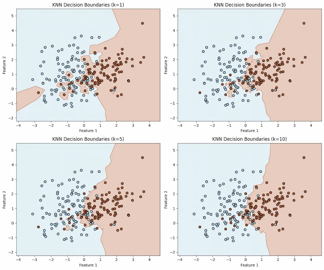
This visualization directly connects to the accuracy plot we discussed.
- The complex boundary at K=1 is likely overfit. It might do perfectly on the training data but perform poorly on new, unseen data.
- The smoother boundaries at K=5 or K=10 are more generalized. They might misclassify a few training points but are more likely to perform well on the test set. If 'K' becomes too large, the boundary might become overly simplistic and performance will drop again (underfitting).
Your task as a machine learning practitioner is to use the accuracy plot to find the 'K' that corresponds to a "just right" decision boundary—not too complex, not too simple.
Conclusion
In this lesson, you've bridged the gap between the theory of K-NN and its practical application. You now have the tools to not only implement the algorithm but also to tune its most important hyperparameter, 'K'.
Key Takeaways:
- K-NN is implemented in scikit-learn using
KNeighborsClassifier. The number of neighbors is set with then_neighborsparameter. - The standard workflow of
.fit()and.predict()applies directly to the K-NN model. - Analyzing the effect of 'K' is a crucial hyperparameter tuning step. A common method is to loop through a range of 'K' values, compute the cross-validated accuracy for each, and plot the results to find the optimal value.
- Changing 'K' directly impacts the complexity of the model's decision boundary, which illustrates the bias-variance trade-off.
Preview of the Next Lesson
Having explored our first classifier, we are now ready to categorize classification models more formally. In the next lesson, we will introduce a fundamental distinction in machine learning: generative vs. discriminative models. Understanding this difference will provide a new framework for thinking about the algorithms we've learned and will set the stage perfectly for our next model, Naive Bayes, which is a classic example of a generative classifier.