PCA with Scikit-learn: Transform and Visualize

The scikit-learn PCA Workflow

Implementing PCA in scikit-learn follows a clear, three-step process. Since you have a solid background with scikit-learn, this should feel very familiar.

Step 1: Standardize the Data

Before applying PCA, it is crucial to scale your data. Remember, PCA's goal is to find directions of maximum variance. If your features are on different scales (e.g., one feature ranges from 0-1 and another from 0-1,000,000), the feature with the larger scale will inherently have a larger variance and will dominate the PCA algorithm, regardless of whether it's truly more "informative".

By standardizing the data—transforming each feature to have a mean of 0 and a standard deviation of 1—we ensure that all features are on a level playing field and contribute equally to the analysis. The StandardScaler from scikit-learn is the perfect tool for this.

Step 2: Apply PCA and Transform the Data

Once the data is scaled, you can apply PCA. This involves two main actions, which scikit-learn conveniently combines into one method:

1. Instantiate PCA: You create an instance of the PCA class, specifying how many principal components you want to keep. For visualization purposes, we typically choose 2 or 3.

   from sklearn.decomposition import PCA
   pca = PCA(n_components=2) 
   

2. Fit and Transform: You use the .fit_transform() method on your scaled data. This single call does two things:
   • fit(): It learns the principal components from the data (i.e., it calculates the directions of maximum variance).
   • transform(): It then projects your original data onto these newly found principal components.

The result is a new array where the number of columns equals n_components.

Step 3: Visualize the Transformed Data

The output of the previous step is your data represented in a new, lower-dimensional space. If you chose n_components=2, you have a 2D representation of your original, higher-dimensional data. You can now create a simple scatter plot using these two new dimensions (Principal Component 1 and Principal Component 2) to visualize your dataset. Often, this reveals patterns, such as clusters, that were hidden in the original feature space.

Guided Walkthrough with StatQuest

The following video provides a concise and practical demonstration of this exact workflow in Python. It's a great way to see these steps in action.

A Complete Code Example: PCA on the Iris Dataset

To solidify your understanding, let's walk through a complete, self-contained example using the classic Iris dataset. This dataset has 4 features, making it impossible to visualize in its entirety. We'll use PCA to project it down to 2 dimensions.

1. Imports and Data Loading

First, we import the necessary libraries and load the Iris dataset, which is conveniently included in scikit-learn.

import pandas as pd
import matplotlib.pyplot as plt
from sklearn.preprocessing import StandardScaler
from sklearn.decomposition import PCA
from sklearn.datasets import load_iris




# Load the dataset
iris = load_iris()
X = iris.data
y = iris.target
target_names = iris.target_names

2. Standardize the Features

As discussed, we scale the 4 features in X.

# Standardizing the features
X_scaled = StandardScaler().fit_transform(X)

3. Perform PCA

We create a PCA object to reduce the data to 2 dimensions and then apply it to our scaled data.

# Apply PCA
pca = PCA(n_components=2)
principalComponents = pca.fit_transform(X_scaled)

4. Create a DataFrame for Plotting

It's often helpful to put the results into a Pandas DataFrame, which makes plotting with labels easier.

# Create a DataFrame with the principal components
principal_df = pd.DataFrame(data = principalComponents, 
                            columns = ['PC 1', 'PC 2'])




# Add the target labels for coloring the plot
final_df = pd.concat([principal_df, pd.DataFrame(y, columns=['target'])], axis=1)

5. Visualize the 2D Projection

Finally, we use matplotlib to create a scatter plot of our two principal components, coloring each point by its flower species.

fig = plt.figure(figsize = (8, 6))
ax = fig.add_subplot(1, 1, 1) 
ax.set_xlabel('Principal Component 1', fontsize = 12)
ax.set_ylabel('Principal Component 2', fontsize = 12)
ax.set_title('2 Component PCA on Iris Dataset', fontsize = 15)

colors = ['r', 'g', 'b']
for target, color in zip(range(len(target_names)), colors):
    indices_to_keep = final_df['target'] == target
    ax.scatter(final_df.loc[indices_to_keep, 'PC 1'],
               final_df.loc[indices_to_keep, 'PC 2'],
               c = color,
               s = 50)
ax.legend(target_names)
ax.grid()
plt.show()

When you run this code, you will get a plot like this:

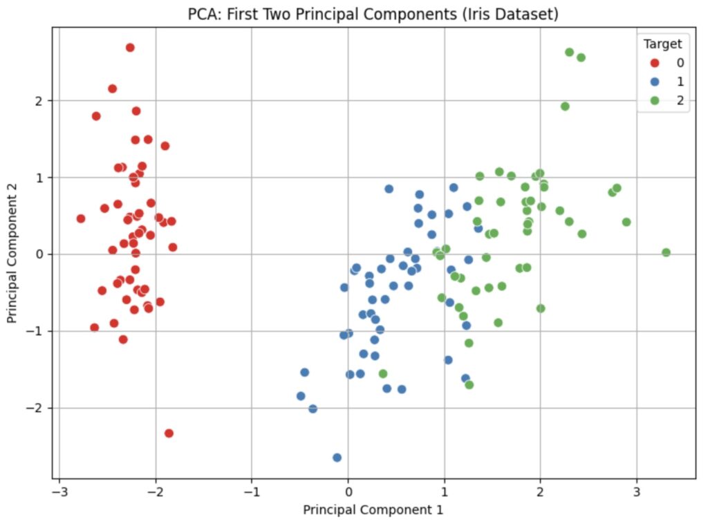
This visualization is powerful. We've taken 4-dimensional data and successfully represented it in 2 dimensions, revealing that the classes are largely separable in this new feature space.

Conclusion

In this lesson, you have learned the practical steps to apply PCA using scikit-learn. You now know how to take a high-dimensional dataset and transform it into a low-dimensional representation suitable for visualization.

Key Takeaways:

• The standard PCA workflow is: Standardize -> Fit/Transform -> Visualize.
• Standardizing features with StandardScaler is a critical prerequisite to prevent features with large scales from dominating the analysis.
• PCA(n_components=k) is used to create a PCA transformer that will reduce the data to k dimensions.
• The .fit_transform() method is a convenient way to both learn the principal components from the data and project the data onto them in one step.
• The resulting principal components can be plotted to visualize the structure of the data, often revealing clusters or patterns.

Preview of the Next Lesson

In our example, we arbitrarily chose to keep 2 components because our goal was 2D visualization. But what if our goal was to reduce dimensions for a machine learning model? How many components should we keep? Is 2 enough? Is 5 too many? In the next lesson, you will learn how to use the explained variance ratio to make an informed decision about the optimal number of principal components to retain.