Feynman Rules for QCD

The Complete QCD Lagrangian

As a starting point, let's write down the full, gauge-fixed Lagrangian for QCD that we established. It's composed of the quark sector, the Yang-Mills sector (gluons), the gauge-fixing term, and the ghost sector.

${\mathcal{L}}_{\text{QCD}}=\underset{\text{Quarks}}{\underbrace{\bar{\psi }(i{\gamma }^{\mu }{D}_{\mu }-m)\psi }}\underset{\text{Yang-Mills}}{\underbrace{-\frac{1}{4}{F}_{\mu \nu }^a{F}_a^{\mu \nu }}}\underset{\text{Gauge-Fixing}}{\underbrace{-\frac{1}{2\xi }({\partial }^{\mu }{A}_{\mu }^a{)}^2}}+\underset{\text{Ghosts}}{\underbrace{{\bar{c}}^a(-{\partial }^{\mu }{D}_{\mu }^{ab})c^b}}$

Here, $D_{\mu }={\partial }_{\mu }-i{g}_s{t}^a{A}_{\mu }^a$ is the covariant derivative in the fundamental representation (acting on quarks), and $D_{\mu }^{ab}={\delta }^{ab}{\partial }_{\mu }+g_s{f}^{abc}{A}_{\mu }^c$ is the covariant derivative in the adjoint representation (acting on ghosts).

The core idea for deriving Feynman rules is to split the Lagrangian into a "free" part (${\mathcal{L}}_0$), containing terms that are quadratic in the fields, and an "interaction" part (${\mathcal{L}}_{\text{int}}$), containing all higher-order terms.

• ${\mathcal{L}}_0$: Describes the free propagation of particles. Its inverse in momentum space gives the propagators.
• ${\mathcal{L}}_{\text{int}}$: Describes the interactions between particles. Its terms correspond directly to the vertices.

Expanding the full Lagrangian gives us the following interaction terms:

1. ${\mathcal{L}}_{q-g}=g_s\bar{\psi }{\gamma }^{\mu }{t}^a{A}_{\mu }^a\psi$ (Quark-gluon interaction)
2. ${\mathcal{L}}_{3g}=-g_s{f}^{abc}({\partial }_{\mu }{A}_{\nu }^a)A^{\mu b}{A}^{\nu c}$ (Three-gluon interaction)
3. ${\mathcal{L}}_{4g}=-\frac{1}{4}{g}_s^2{f}^{abe}{f}^{cde}{A}_{\mu }^a{A}_{\nu }^b{A}^{\mu c}{A}^{\nu d}$ (Four-gluon interaction)
4. ${\mathcal{L}}_{\text{ghost}-g}=g_s{f}^{abc}{\bar{c}}^a{A}_{\mu }^b({\partial }^{\mu }{c}^c)$ (Ghost-gluon interaction, after integration by parts)

Propagators: The Free Particle Motion

Propagators represent the amplitude for a particle to travel from one spacetime point to another. In momentum space, the propagator is $i$ times the inverse of the kinetic operator found in ${\mathcal{L}}_0$.

1. Quark Propagator

The free quark Lagrangian is ${\mathcal{L}}_{\text{quark},0}=\bar{\psi }(i/\partial -m)\psi$. In momentum space (${\partial }_{\mu }\to -i{p}_{\mu }$), the kinetic operator is $(/p-m)$. The propagator is therefore:

The ${\delta }_{ij}$ indicates that color is conserved during propagation; a quark does not change its color while traveling freely.

2. Gluon Propagator

The free gluon Lagrangian, including the gauge-fixing term, is ${\mathcal{L}}_{\text{gluon},0}+{\mathcal{L}}_{\text{GF}}$. After some algebra and integration by parts, the quadratic term in momentum space can be written as $\frac{1}{2}{A}_{\mu }^a(k)K_{ab}^{\mu \nu }{A}_{\nu }^b(-k)$, where the kinetic operator is:
$K_{ab}^{\mu \nu }=[-k^2{g}^{\mu \nu }+(1-\frac{1}{\xi })k^{\mu }{k}^{\nu }]{\delta }_{ab}$
Inverting this tensor gives the gluon propagator. A common and convenient choice is the Feynman gauge, where $\xi =1$. In this gauge, the propagator simplifies significantly:

The ${\delta }_{ab}$ shows that, like quarks, gluons do not change their color charge when propagating freely.

3. Ghost Propagator

The free ghost Lagrangian from ${\mathcal{L}}_{\text{ghost}}$ is ${\mathcal{L}}_{\text{ghost},0}={\bar{c}}^a(-{\partial }^2)c^a$. In momentum space, the kinetic operator is simply $p^2$. The ghost propagator is that of a simple massless scalar, but with color indices:

Vertices: The Interactions

Vertices are derived from the terms in ${\mathcal{L}}_{\text{int}}$. The rule for each vertex is obtained by writing the interaction term in momentum space and multiplying by $i$.

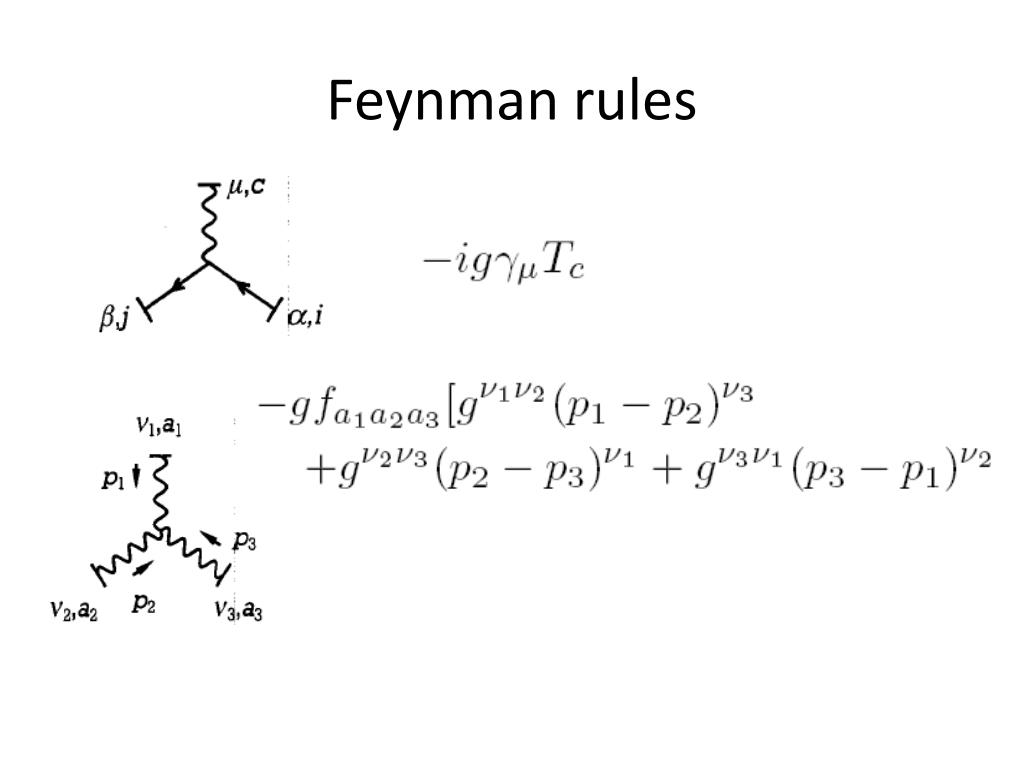
1. Quark-Gluon Vertex

From ${\mathcal{L}}_{q-g}=g_s\bar{\psi }{\gamma }^{\mu }{t}^a{A}_{\mu }^a\psi$, we get the rule for a quark interacting with a gluon. This is the fundamental interaction of QCD.
The vertex factor is: $i{g}_s{\gamma }^{\mu }{t}_{ij}^a$.

2. Three-Gluon Vertex

This vertex arises from the gluon self-interaction term ${\mathcal{L}}_{3g}$, which is a direct consequence of the non-Abelian nature of QCD. It involves three gluon fields and a derivative. After accounting for permutations of the fields, we arrive at the vertex rule. For three gluons with colors $a,b,c$, Lorentz indices $\mu ,\nu ,\rho$, and incoming momenta $p,q,k$, the vertex is:
$g_s{f}^{abc}\left[g^{\mu \nu }(p-q{)}^{\rho }+g^{\nu \rho }(q-k{)}^{\mu }+g^{\rho \mu }(k-p{)}^{\nu }\right]$

3. Four-Gluon Vertex

This arises from the ${\mathcal{L}}_{4g}$ term. It is a contact interaction of four gluons. Its structure is quite complex, involving two structure constants and three terms corresponding to the different ways of pairing the Lorentz indices:
$-i{g}_s^2\left[f^{abe}{f}^{cde}(g^{\mu \rho }{g}^{\nu \sigma }-g^{\mu \sigma }{g}^{\nu \rho })+f^{ace}{f}^{bde}(g^{\mu \beta }{g}^{\rho \sigma }-g^{\mu \sigma }{g}^{\beta \rho })+f^{ade}{f}^{bce}(g^{\mu \rho }{g}^{\beta \sigma }-g^{\mu \beta }{g}^{\rho \sigma })\right]$

4. Ghost-Gluon Vertex

Finally, from ${\mathcal{L}}_{\text{ghost}-g}$, we find the vertex describing the interaction between a ghost, an anti-ghost, and a gluon. Let the incoming gluon have color $a$ and momentum $q$, and let the ghost line carry momentum $p$ (flowing out of the vertex). The vertex rule is:
$g_s{f}^{abc}{p}^{\mu }$
Notice the momentum dependence, which comes from the derivative in the ghost Lagrangian. The arrow on the ghost line is crucial; by convention, momentum $p$ is that of the ghost, which flows in the direction of the arrow.

Summary of Feynman Rules for QCD

We have now derived all the pieces. The following resources provide a clear, graphical summary of these rules.

To visualize some of these key interactions, consider the following diagram:

The Physical Role of Ghost Vertices

We introduced ghosts as a mathematical necessity to make the path integral well-defined. But what is their physical role? As we discussed in the previous lesson, they ensure the theory is unitary. When we calculate loop diagrams, the unphysical gluon polarizations that circulate in the loops are precisely cancelled by diagrams containing ghost loops.

The following reading provides an excellent explicit demonstration of this cancellation for the process $q\bar{q}\to gg$. It shows that to get the correct physical result when summing over gluon polarizations, you must subtract a "ghost contribution". This isn't an ad-hoc procedure; it is the direct consequence of the Feynman rules we just derived.

Conclusion

In this lesson, we have translated our complete QCD Lagrangian into a concrete set of Feynman rules. These rules are the cornerstone of perturbative QCD.

Key Takeaways:

• Feynman rules are derived by splitting the Lagrangian into a free part (for propagators) and an interaction part (for vertices).
• The quark propagator is similar to the Dirac case, but carries color indices.
• The gluon propagator is simple in Feynman gauge ($\xi =1$), representing a massless, color-carrying vector particle.
• The ghost propagator is that of a massless, color-carrying scalar field.
• QCD features four fundamental interaction vertices: the quark-gluon vertex, the three-gluon vertex, the four-gluon vertex, and the ghost-gluon vertex.
• The gluon self-interactions and the ghost interaction are unique features of non-Abelian gauge theories.

Preview of the Next Lesson:

Now that we have the full set of rules, you might think we are ready to calculate a scattering amplitude. However, there is one more crucial piece of algebra to master: handling the color indices. Every vertex involves either a Gell-Mann matrix $t^a$ or a structure constant $f^{abc}$, and every internal line has a Kronecker delta ${\delta }_{ij}$ or ${\delta }_{ab}$. To compute a physical, unpolarized cross-section, we must sum over all final state colors and average over all initial state colors. In the next lesson, we will learn how to define and compute color factors for QCD diagrams using the algebraic properties of the SU(3) generators.