QCD Beta Function & Asymptotic Freedom

Hello! In our last lesson, we performed a complete tree-level calculation for quark-quark scattering, seeing how the kinematic structures familiar from QED are dressed with the non-trivial algebra of color. That calculation gave us a leading-order snapshot of the strong interaction.

Today, we take a significant step forward by exploring what happens when we include quantum fluctuations through loop diagrams. This will lead us to one of the most profound discoveries in theoretical physics: asymptotic freedom. We will calculate the one-loop beta function for QCD, which governs how the strength of the strong force changes with energy. This result not only explains why the perturbative methods we've been using are valid at high energies but also hints at the phenomenon of quark confinement at low energies.

The Running of Couplings: A Tale of Two Theories

You'll recall from our study of QED that loop corrections lead to the concept of a "running" coupling constant. The strength of the electromagnetic interaction, $α$ , is not truly a constant but changes with the energy scale of the process. This is due to vacuum polarization: virtual electron-positron pairs pop out of the vacuum and screen the bare electric charge, making the observed charge smaller at larger distances (lower energies).

In QCD, a similar screening effect occurs due to virtual quark-antiquark pairs. However, QCD has a unique feature not present in QED: gluons, the force carriers themselves, are colored and thus interact with each other. This gluon self-interaction leads to a competing effect called anti-screening.

To get a clear physical picture of this, let's watch a brief segment from a lecture by Alex Flournoy.

Particle Physics (2018) Topic 28: Renormalization in QCD, Effective Field Theories and Strings

This video provides an excellent conceptual overview of renormalization in QCD, contrasting it with QED. It explains the physical origin of screening and anti-screening without getting into the mathematical details just yet.

Watch the section from 30:49 to 43:30. Focus on the distinction between the quark-loop contribution (screening) and the gluon-loop contribution (anti-screening). Pay attention to the argument about which effect dominates based on the number of colors and flavors.

As the video explains, we have two competing effects:

Screening: Virtual quark-antiquark loops screen the color charge, similar to how $e^{+} e^{-}$ loops screen electric charge. This effect tends to make the strong coupling $α_{s}$ increase at high energy (short distances).
Anti-screening: Virtual gluon loops (and ghost loops, which we need for gauge consistency) have the opposite effect. You can think of this as the color charge "leaking out" and spreading over a larger area, effectively making the interaction weaker at high energy.

The diagrams responsible for these effects on the gluon propagator are shown below.

One-Loop Contributions to the Gauge Boson Propagator — Figure 1: One-loop corrections to the gluon propagator. (a) The quark loop, which causes screening. (b) The gluon loop and (c) the ghost loop, which together cause anti-screening.

Which effect wins? The answer lies in a detailed calculation. Our goal is to compute the beta function, $β (α_{s})$ , which is defined as the rate of change of the coupling with the energy scale $μ$ :

β (α_{s}) = \frac{d α _{s}}{d ( ln μ )}

The sign of the beta function will tell us whether the coupling grows or shrinks with energy.

The Calculation: One-Loop Renormalization of QCD

The calculation of the beta function requires us to compute the ultraviolet (UV) divergences from one-loop diagrams and absorb them into renormalization constants. We will use dimensional regularization, where calculations are performed in $d = 4 - 2 ϵ$ spacetime dimensions to regulate the divergent integrals. The divergences then appear as poles in $1/ ϵ$ .

The strategy is as follows:

Relate the "bare" fields ( $ψ_{B}, A_{B}$ ) and coupling ( $g_{B}$ ) in the original Lagrangian to their "renormalized," physically measurable counterparts ( $ψ_{R}, A_{R}, g_{R}$ ) via renormalization constants $Z_{i}$ . $ψ_{B} = Z_{2}^{1/2} ψ_{R}, A_{B}^{μ} = Z_{3}^{1/2} A_{R}^{μ}, g_{B} = μ^{ϵ} Z_{g} g_{R}$ The factor $μ^{ϵ}$ is introduced to keep the renormalized coupling $g_{R}$ dimensionless in $d$ dimensions.
Calculate the one-loop corrections to the quark propagator, gluon propagator, and quark-gluon vertex to find the divergent parts of $Z_{2}$ , $Z_{3}$ , and $Z_{1}$ (the vertex renormalization constant).
Use the Slavnov-Taylor identities (the non-Abelian version of Ward identities) which enforce gauge invariance, leading to the relation: $Z_{g} = \frac{Z _{1}}{Z _{2} Z _{3}}$
The fundamental principle of renormalization is that the bare theory must be independent of our arbitrary choice of renormalization scale $μ$ . By requiring $\frac{d g _{B}}{d μ} = 0$ , we can derive the beta function for $g_{R}$ .

This is a formidable calculation. We will not perform every integral from scratch. Instead, we'll use a detailed reference to understand the structure and key results of each step. The following resource provides a complete, self-contained derivation.

Introduction to perturbative QCD

The following sections from Carlo Oleari's lecture notes, 'Introduction to perturbative QCD', walk through the entire one-loop calculation. We will focus on the main results that build up to the beta function.

Your task is to follow the logic of the calculation in Chapter 5. You don't need to re-derive every line, but focus on understanding how the pieces fit together. Section 5.1 (Gluon self-energy): Read through this section to see how the contributions from the fermion loop (Eq. 5.3), gluon loop (Eq. 5.5), and ghost loop (Eq. 5.8) are summed. The final result for the gluon field renormalization constant, Z_3, is given in Eq. (5.13). Note the opposite signs of the C_A and n_f T_F terms! Sections 5.2 & 5.3 (Quark self-energy and Vertex correction): Skim these sections to find the results for Z_2 (Eq. 5.14) and Z_1^{-1} (Eq. 5.27). Notice that (Z_1 eq Z_2), unlike in QED. Section 5.3 (continued): The end of this section (from Eq. 5.29 onwards) is crucial. It shows how Z_1, Z_2, Z_3 are combined to find the coupling renormalization constant Z_g in Eq. (5.35). Section 5.4 (The running coupling and β function): This is the final step. Read this section carefully. It shows how the requirement that the bare coupling is independent of \mu leads to the beta function (Eq. 5.42) and the final expression for the running coupling \alpha_s(\mu^2) (Eq. 5.44).

Summary of the Calculation

Let's distill the key results from the reading. The one-loop renormalization constants are found to have divergent parts (proportional to $1/ ϵ$ ):

Gluon Renormalization ( $Z_{3}$ ):
$Z_{3} = 1 + \frac{α _{s}}{4 π} \frac{1}{ϵ} (\frac{5}{3} C_{A} - \frac{4}{3} n_{f} T_{F})$
This is the heart of the matter. $C_{A} = N_{c} = 3$ is the adjoint Casimir, coming from the gluon/ghost loops (anti-screening). $n_{f}$ is the number of quark flavors, and $T_{F} = 1/2$ comes from the quark loops (screening). The positive sign of the $C_{A}$ term and the negative sign of the $n_{f}$ term reflect the competition we discussed.
Quark Renormalization ( $Z_{2}$ ):
$Z_{2} = 1 - \frac{α _{s}}{4 π} \frac{1}{ϵ} C_{F}$
Where $C_{F} = \frac{N _{c}^{2} - 1}{2 N _{c}} = \frac{4}{3}$ is the fundamental Casimir.
Vertex Renormalization ( $Z_{1}$ ):
$Z_{1} = 1 - \frac{α _{s}}{4 π} \frac{1}{ϵ} (C_{F} + C_{A})$

From these, the coupling renormalization constant $Z_{g} = Z_{1} Z_{2}^{- 1} Z_{3}^{- 1/2}$ is computed. To first order in $α_{s}$ , this gives:

Z_{g} = 1 - \frac{α _{s}}{4 π} \frac{1}{ϵ} (\frac{11}{6} C_{A} - \frac{2}{3} n_{f} T_{F})

Finally, demanding that the bare coupling $g_{B}$ is independent of $μ$ yields the beta function. In terms of $α_{s} = g_{R}^{2} /4 π$ , the result is:

β (α_{s}) = μ^{2} \frac{d α _{s}}{d μ ^{2}} = - \frac{α _{s}^{2}}{2 π} (\frac{11}{3} N_{c} - \frac{2}{3} n_{f})

This is one of the most important formulas in the Standard Model.

Test your understanding!

For QED, the beta function is positive: $β (α) \approx + \frac{2 α ^{2}}{3 π}$ . Compare the general structure of the QED and QCD beta functions. What is the crucial term in the QCD beta function that has no analogue in QED, and why is it physically present?

Show answer

The QED beta function arises purely from fermion loops (screening). The QCD beta function has a term $- \frac{2}{3} n_{f}$ which is analogous to the QED case (it comes from quark loops), but it also has the term $+ \frac{11}{3} N_{c}$ . This $N_{c}$ term, with its overall negative sign in the beta function, is the crucial difference. It originates from the gluon and ghost loops (as seen in the calculation of $Z_{3}$ ). Physically, it is present because gluons carry color charge and self-interact, a feature absent in QED where photons are electrically neutral. This term is responsible for anti-screening.

Asymptotic Freedom and Confinement

Let's analyze our result for QCD, where $N_{c} = 3$ . The number of quark flavors $n_{f}$ that are light enough to contribute to the loops depends on the energy scale, but for typical high-energy experiments, all 6 are relevant.

β (α_{s}) = - \frac{α _{s}^{2}}{2 π} (\frac{11}{3} (3) - \frac{2}{3} (6)) = - \frac{α _{s}^{2}}{2 π} (11 - 4) = - \frac{7 α _{s}^{2}}{2 π}

The crucial result is that the beta function is negative.

What does this mean?

A negative $β (α_{s})$ implies that $\frac{d α _{s}}{d ( l n μ )} < 0$ . The coupling constant $α_{s}$ decreases as the energy scale $μ$ increases.
This phenomenon is called asymptotic freedom. At very high energies or, equivalently, very short distances (e.g., inside a proton during a high-energy collision), quarks and gluons behave almost as if they are free, non-interacting particles. This is why perturbative QCD calculations, like the one we did in the last lesson, are so successful in describing high-energy phenomena like jet production.
Conversely, as the energy scale decreases (or distance increases), $α_{s}$ grows. At an energy scale known as $Λ_{QC D} \approx 200$ MeV, the perturbative formula diverges, and the coupling becomes enormous. This suggests that the force between quarks does not fall off with distance but instead becomes stronger, leading to the phenomenon of confinement—the fact that we never observe isolated free quarks or gluons, only color-neutral hadrons (mesons and baryons).

This behavior is precisely what is observed in experiments.

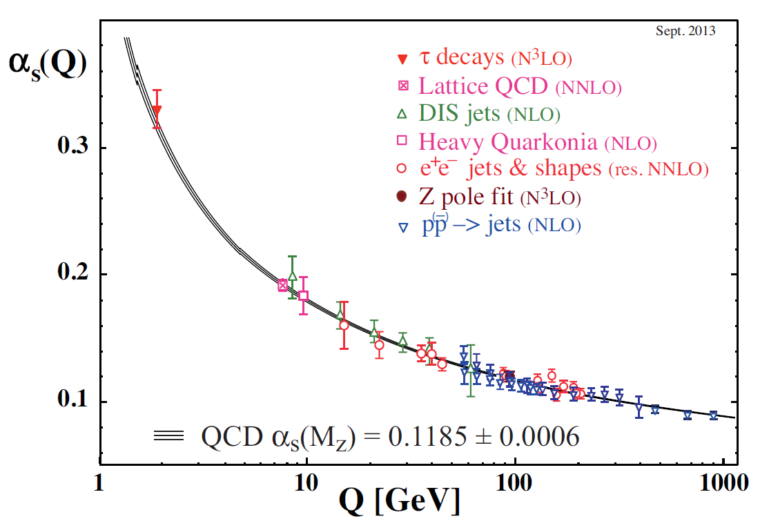
Running of the Strong Coupling Constant α_s(Q) — Figure 2: A summary of experimental measurements of $\alpha_s$ at various energy scales $Q$. The data clearly shows $\alpha_s$ decreasing as energy increases, a spectacular confirmation of the theoretical prediction of asymptotic freedom. The solid line is the theoretical fit from QCD. (Image credit: Particle Data Group)

The discovery of asymptotic freedom in non-Abelian gauge theories by David Gross, Frank Wilczek, and David Politzer in 1973 was a monumental achievement that established QCD as the correct theory of the strong interaction, earning them the 2004 Nobel Prize in Physics.

Conclusion

Key Takeaways:

Renormalization of QCD reveals that the strong coupling constant $α_{s}$ "runs" with energy scale $μ$ .
Unlike in QED where vacuum polarization leads only to charge screening, QCD features a competition between screening (from quark loops) and anti-screening (from gluon self-interaction loops).
The calculation of the one-loop beta function shows that for the number of flavors in our universe, anti-screening wins.
The QCD beta function is negative: $β (α_{s}) = - \frac{α _{s}^{2}}{2 π} (\frac{11}{3} N_{c} - \frac{2}{3} n_{f}) < 0$ .
This negative sign implies asymptotic freedom: $α_{s}$ decreases at high energies, allowing for perturbative calculations.
It also implies that $α_{s}$ grows at low energies, providing a basis for understanding quark confinement.

You have now worked through the calculation and physical reasoning behind one of the deepest and most celebrated results in modern physics.

Preview of the Next Lesson:

We have reached the pinnacle of what we can do with spontaneous symmetry breaking in Abelian theories. To build the Standard Model, we need to combine this idea with the non-Abelian gauge theories we've just studied. In the next lesson, we will begin our journey into the electroweak sector by analyzing the spontaneous breaking of a global continuous symmetry and deriving the famous Goldstone's theorem.

Recommended resources

The Running of Couplings: A Tale of Two Theories

The Calculation: One-Loop Renormalization of QCD

Summary of the Calculation

Asymptotic Freedom and Confinement

Conclusion