Hello! Welcome to the second module of our course on Quantum Field Theory. In the first module, we successfully constructed a consistent, causal, relativistic quantum theory for free scalar particles. While this was a monumental achievement, the real world is filled with interactions. Particles are not isolated; they scatter, decay, and bind together. To describe these phenomena, we must venture into the realm of interacting fields.
This lesson marks our first step in that direction. We will build upon the foundation of the free theory to develop a framework for handling interactions perturbatively. This is the cornerstone of most calculations in QFT, from particle collider predictions to condensed matter phenomena.
Our learning outcome for today is to: Formulate the interaction picture and derive the Dyson series for the time-evolution operator in φ⁴ theory.
We'll start by introducing the simplest interacting field theory, $\phi^4$ theory. We'll then develop a crucial tool, the interaction picture, which allows us to separate the "easy" free part of the theory from the "hard" interacting part. Finally, we will derive the famous Dyson series, a formal solution for time evolution in an interacting theory, which will be our primary tool for calculations in the lessons to come.
1. Introducing Interactions: The $\lambda\phi^4$ Theory
So far, our Lagrangian for the real scalar field has been:
This describes a "free" theory because the Euler-Lagrange equation it produces—the Klein-Gordon equation—is linear. Its solutions can be superposed, and the particles described by the field (quanta) pass through each other without any effect.
To introduce interactions, we need to add non-linear terms to the Lagrangian. The simplest, Lorentz-invariant, and renormalizable interaction term we can add is a quartic self-interaction. This gives us the Lagrangian for $\lambda\phi^4$ theory:
Here, $\lambda$ is a dimensionless coupling constant that measures the strength of the interaction. The $4!$ is a conventional factor that will simplify our calculations later.
The new equation of motion is:
This equation is non-linear. The beautiful plane-wave expansion we used for the free field is no longer a solution. We cannot solve this theory exactly. Our only hope, for small $\lambda$, is perturbation theory.
2. The Interaction Picture
Perturbation theory requires us to split the Hamiltonian into a solvable part and a small perturbation. For our theory, the split is natural:
where $H_0$ is the familiar free Hamiltonian and $H_I = \int d^3x \frac{\lambda}{4!}\phi^4$ is the interaction Hamiltonian.
The challenge is that the Schrödinger picture, where states evolve with the full Hamiltonian $H$, is too complicated. The Heisenberg picture, where operators evolve with $H$, is equally difficult. We need a hybrid approach: the interaction picture.
The core idea is to let the operators evolve according to the simple free Hamiltonian $H_0$, while the states evolve due to the "difficult" interaction Hamiltonian $H_I$.
The interaction picture of quantum mechanics
For a concise conceptual overview of the interaction picture and how it fits between the Schrödinger and Heisenberg pictures, please watch this short video by Jonathon Riddell.
Watch from 03:34 to 06:24. This segment defines the states and operators in the interaction picture and derives the key equation of motion for the state vector.
Now, let's formalize this. Given your background in advanced quantum mechanics, the following derivation should feel familiar. We will work in natural units ($\hbar=c=1$) from now on.
The following text from David Tong's renowned QFT lecture notes provides a clear and rigorous derivation of the interaction picture. It formally defines the states and operators and derives the equation that governs the time evolution of states.
Please read section 3.1, 'The Interaction Picture' (pages 50-51), stopping before section 3.1.1. Pay close attention to equations (3.11) through (3.14), which define the picture and culminate in the Schrödinger equation for interaction picture states.
To summarize the key results from these resources:
- States in the interaction picture are related to Schrödinger states by: $|\psi_I(t)\rangle = e^{iH_0 t} |\psi_S(t)\rangle$.
- Operators are related by: $O_I(t) = e^{iH_0 t} O_S e^{-iH_0 t}$. Notice this is just the Heisenberg evolution under the free Hamiltonian.
- The time evolution of states is governed by the Schrödinger-like equation: where $H_I(t) = e^{iH_0 t} H_I e^{-iH_0 t}$ is the interaction Hamiltonian in the interaction picture.
This is a powerful result. The operators, including our field $\phi_I(x)$, now evolve according to the free theory. This means we can still use our familiar free field expansion for $\phi_I(x)$! The complexity of the interaction has been moved entirely into the evolution of the state vectors.
3. Solving for Time Evolution: The Dyson Series
Our next task is to solve the evolution equation for the states. Let's define a unitary time-evolution operator $U(t, t_0)$ that evolves states from time $t_0$ to $t$:
Substituting this into the equation of motion gives a differential equation for the operator $U(t, t_0)$:
If $H_I(t)$ were just a function, or if it commuted with itself at different times ($[H_I(t_1), H_I(t_2)] = 0$), the solution would be a simple exponential. However, this is generally not true for operator Hamiltonians. This non-commutativity is the central difficulty.
The solution is an iterative one, leading to what is known as the Dyson series. The derivation is a cornerstone of perturbation theory.
Quantum Theory, Lecture 4.5: Time Evolution Operator. Dyson Series. Time-Ordered Exponential.
The following lecture by Alexander Maloney provides an excellent, pedagogical derivation of the Dyson series from first principles. It's framed in the context of a general time-dependent Hamiltonian in quantum mechanics, which is exactly the problem we face with H_I(t).
Please watch from 28:10 to 55:34. This long segment is the core of today's lesson. It will walk you through: Why the simple exponential solution fails for time-dependent, non-commuting Hamiltonians (28:10 - 41:12). The iterative construction of the solution and the introduction of the time-ordering operator, leading to the Dyson series (41:12 - 55:34). Your strong QM background will be very helpful here.
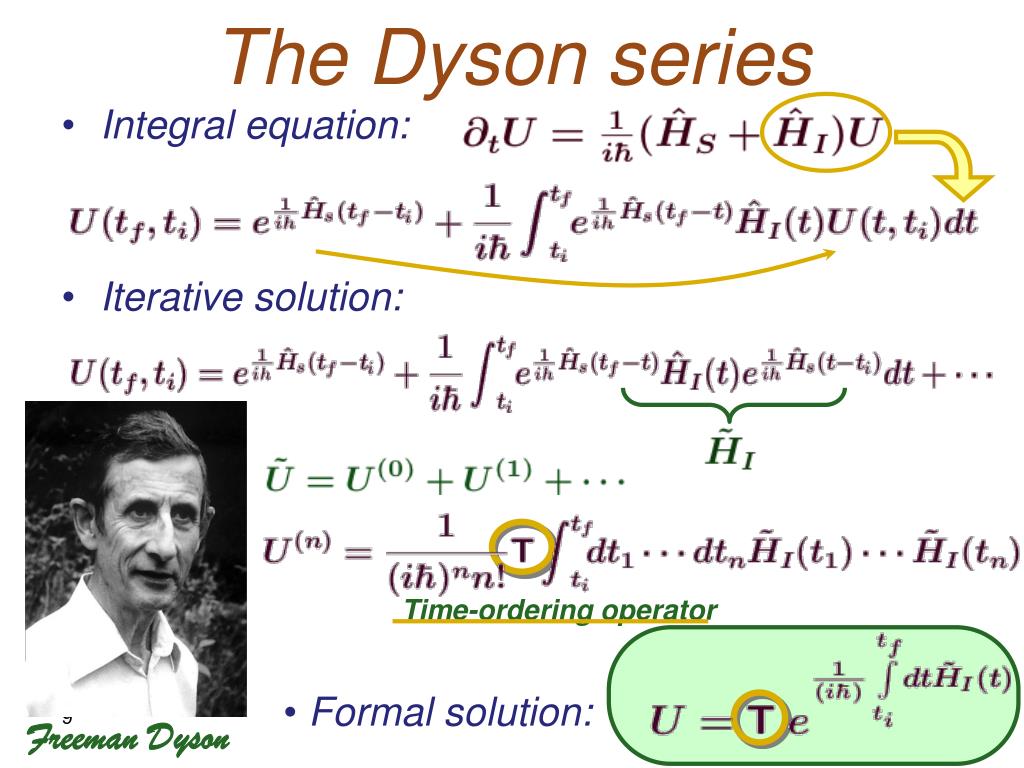
Let's recap the result of this beautiful derivation. The solution for the time-evolution operator is given by the Dyson formula:
where $T$ is the time-ordering operator. It ensures that when the exponential is expanded as a series, the operators $H_I(t')$ are always ordered with later times to the left.
The series expansion, which is what we actually use in calculations, is:
Test your understanding!
Suppose you are calculating the second-order term in the Dyson series: $$ U^{(2)}(t, t_0) = (-i)^2 \int_{t_0}^t dt_1 \int_{t_0}^{t_1} dt_2 H_I(t_1) H_I(t_2) $$ Using the time-ordering operator, this can be rewritten with symmetric integration limits: $$ U^{(2)}(t, t_0) = \frac{(-i)^2}{2!} \int_{t_0}^t dt_1 \int_{t_0}^t dt_2 \, T\big( H_I(t_1) H_I(t_2) \big) $$ Why is the factor of $1/2!$ necessary in the second form but not the first?Show answer
The first form has nested integrals with limits $t_0 \le t_2 \le t_1 \le t$. This restricts the integration domain to a specific "triangle" in the $t_1$-$t_2$ plane, where $t_1$ is always later than $t_2$. The time ordering is therefore enforced by the integration limits.
The second form integrates over the full "square" region where both $t_1$ and $t_2$ run from $t_0$ to $t$. This square region includes both the case $t_1 > t_2$ and $t_2 > t_1$. The time-ordering operator $T$ handles putting the operators in the correct order for each point in the domain. Because we are integrating over a domain that is twice as large as the original triangular domain (by symmetry), we must divide by $2$ (or $2!$) to get the correct result. The same logic applies with a factor of $1/n!$ for the $n$-th order term.
4. The Dyson Series for $\phi^4$ Theory
We can now put everything together for our specific theory. The interaction Hamiltonian in the Schrödinger picture is:
In the interaction picture, this becomes:
where $\phi_I(\vec{x}, t)$ is the free field operator that evolves with $H_0$.
Substituting this into the Dyson formula gives us the time-evolution operator for $\phi^4$ theory:
This expression is the starting point for all of perturbative QFT. In scattering experiments, we are interested in what happens to a state of incoming particles from the infinite past ($t_0 \to -\infty$) as it evolves to a state of outgoing particles in the infinite future ($t \to +\infty$). This transition is described by the S-matrix (Scattering matrix), which is defined as $S \equiv U(+\infty, -\infty)$.
Conclusion
In this lesson, we have built the essential machinery for tackling interacting quantum fields. We have moved from the clean but simple world of free fields into the complex but realistic domain of interactions.
Key Takeaways:
- Interactions are introduced by adding non-linear terms to the Lagrangian, with $\lambda\phi^4$ being the canonical example for a self-interacting scalar field.
- The interaction picture is a hybrid framework where operators evolve with the free Hamiltonian ($H_0$) and states evolve with the interaction Hamiltonian ($H_I(t)$). This allows us to continue using the free field expansion for our field operators.
- The time evolution of states in the interaction picture is not trivial because $H_I(t)$ does not commute with itself at different times.
- The formal solution is the Dyson series, an expansion of the time-ordered exponential of the integrated interaction Hamiltonian: $U(t, t_0) = T \exp(-i \int_{t_0}^t H_I(t') dt')$.
- This series provides a systematic way to calculate the effects of interactions order by order in the coupling constant $\lambda$.
We now have a formal expression for how states evolve under interactions. But this expression involves products of many field operators inside a time-ordering symbol. How do we evaluate these? This is where the real calculational power of QFT begins to emerge.
Preview of the Next Lesson:
In our next lesson, we will learn how to tame the Dyson series. We will derive Wick's Theorem, a powerful combinatorial tool that allows us to systematically break down the time-ordered products of many field operators into sums of simple, calculable terms called propagators and normal-ordered products. This theorem is the direct link between the Dyson series and the famous Feynman diagrams.