Deriving the Differential Cross-Section in the CM Frame

Hello! Welcome back to our course on Quantum Field Theory.

In our last lesson, we calculated our first scattering amplitude, finding that for tree-level $2 \to 2$ scattering in $ϕ^{4}$ theory, the invariant matrix element is simply $M = - λ$ . We also introduced the Mandelstam variables as a powerful way to describe the kinematics of such processes.

However, $M$ is a theoretical construct. How does it relate to something that can actually be measured in a particle accelerator? The answer lies in the concept of the scattering cross-section. Today, we will bridge this gap between theory and experiment.

This lesson is dedicated to deriving the crucial formula that connects the invariant matrix element $M$ to the differential cross-section for a $2 \to 2$ scattering process. We will perform the derivation in the center-of-mass frame, which is the most convenient reference frame for both theoretical calculations and many collider experiments.

1. What is a Cross-Section?

Imagine you are firing a beam of particles (projectiles) at a stationary target. The total cross-section, $σ$ , represents the effective "area" of each target particle that the projectiles must hit to cause a scattering event of any kind.

However, physicists are usually interested in more detail. They don't just want to know if a scattering happened, but also where the particles went. This is quantified by the differential cross-section, $d σ / d Ω$ . It represents the effective target area that scatters incoming particles into a specific, infinitesimally small solid angle $d Ω$ .

Scattering Geometry and Solid Angle — This diagram illustrates the concept of a differential cross-section. Incident particles hitting the small annular area $dA = b \, db \, d\phi$ are scattered into the solid angle $d\Omega = \sin\theta \, d\theta \, d\phi$. The differential cross-section, $d\sigma/d\Omega$, is the proportionality factor between these two quantities.

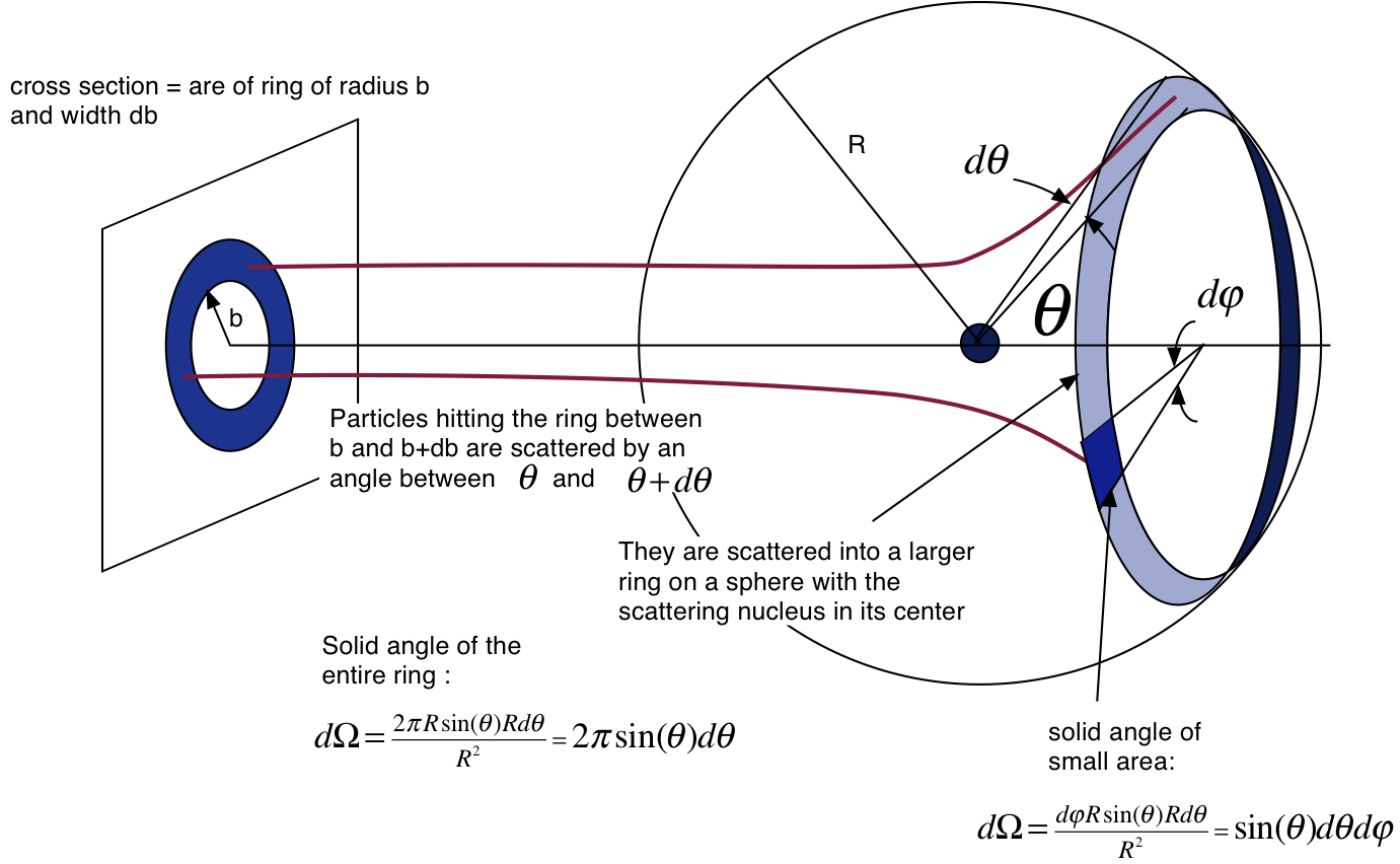
Our goal is to derive a formula for $d σ / d Ω$ in terms of the invariant amplitude $M$ that we learned how to calculate in the previous lessons.

To get a better feel for the concept, the following video gives a clear conceptual overview.

Scattering Cross Sections In Quantum Field Theory | Differential Scattering Cross Section

Please watch the beginning of this video from Dietterich Labs for a conceptual introduction to total and differential scattering cross-sections.

Watch from 2:00 to 7:30. Focus on how the idea of a classical cross-section (an area) is extended to a probabilistic, effective area in quantum mechanics, and how the differential cross-section provides more detailed information about the scattering angles.

2. From S-Matrix to a General Cross-Section Formula

The full derivation is quite involved, as it requires carefully considering the initial state (as localized wave packets, not infinite plane waves), the time evolution via the S-matrix, and the measurement of the final state. We'll be guided by a detailed lecture that walks through this process. The key idea is to calculate the probability of a transition from an initial state $∣ i ⟩$ to a final state $∣ f ⟩$ and relate it to the cross-section.

The transition probability $P_{i \to f}$ is proportional to the square of the S-matrix element, $∣ ⟨ f ∣ S ∣ i ⟩ ∣^{2}$ . We are interested in scattering events, so we use the transition matrix $T$ , defined by $S = I + i T$ . The invariant matrix element $M$ is then defined by factoring out momentum conservation from the T-matrix element:

⟨ f ∣ i T ∣ i ⟩ = (2 π)^{4} δ^{4} (P_{f} - P_{i}) M_{f i}

The derivation then proceeds by:

Writing the initial state as a superposition of momentum eigenstates (wave packets) for two particles, with one packet having a transverse offset (the impact parameter).
Calculating the transition probability to a set of final states with specific momenta.
Integrating this probability over all possible impact parameters to find the total probability for scattering to occur for a given beam configuration.
Dividing by the incident particle flux to obtain the cross-section.

The following video provides a rigorous derivation of the general formula. It's mathematically dense, but it's a classic and important calculation in QFT. Given your background, you should be able to follow the main steps.

Quantum Field Theory I - Lecture 11

This lecture from IFT-UNESP provides a detailed derivation connecting the S-matrix to the cross-section. We will follow its logic closely.

Watch from 5:39 to 56:26. This is a long and detailed segment. Don't worry about memorizing every single step. Instead, focus on understanding the logical flow: (5:39 - 15:57) How the probability for a single event is generalized to a cross-section by integrating over the impact parameter b. (15:57 - 39:12) How the S-matrix elements are replaced by the invariant matrix elements M, and how the many integrals over initial state momenta are handled using delta functions. The result of this complex integration is physically intuitive: the initial state wave packets are effectively treated as plane waves with definite momenta. (39:12 - 56:26) How the initial, frame-dependent kinematic pre-factor is rewritten into a Lorentz-invariant form known as the Møller invariant flux.

After this lengthy derivation, one arrives at a master formula for the differential cross-section for a process where two initial particles (momenta $p_{1}, p_{2}$ ) scatter into $n$ final particles (momenta $q_{k}$ ):

d σ = \frac{1}{4 ( p _{1} \cdot p _{2} ) ^{2} - m _{1}^{2} m _{2}^{2}} (k = 1 \prod n \frac{d ^{3} q _{k}}{( 2 π ) ^{3} 2 E _{k}}) ∣ M ∣^{2} (2 π)^{4} δ^{4} (p_{1} + p_{2} - k = 1 \sum n q_{k})

Let's break this down:

The Flux Factor: The term $4 (p_{1} \cdot p_{2})^{2} - m_{1}^{2} m_{2}^{2}$ is the Lorentz-invariant Møller flux. In a frame where the particles collide head-on, it simplifies to $4 E_{1} E_{2} ∣ v_{1} - v_{2} ∣$ , which is proportional to the rate at which incoming particles cross a unit area.
The Phase Space Factor: The product of $d^{3} q_{k} / ((2 π)^{3} 2 E_{k})$ is the Lorentz-Invariant Phase Space (LIPS) element for the final state particles. It represents the number of available final states.
The Matrix Element: $∣ M ∣^{2}$ is the squared invariant amplitude we calculate from Feynman diagrams. It contains all the dynamics of the interaction.
The Delta Function: This enforces overall four-momentum conservation.

3. Specializing to 2→2 Scattering in the Center-of-Mass Frame

Our goal is to find the differential cross-section with respect to the solid angle, $d σ / d Ω$ , for a $2 \to 2$ process. We will work in the Center-of-Mass (CM) frame, which is defined by $p_{1} + p_{2} = 0$ .

In this frame, the kinematics are simplified:

Initial state: $p_{1} = p$ , $p_{2} = - p$ . Total energy $E_{c m} = E_{1} + E_{2}$ .
Final state: By momentum conservation, $q_{1} + q_{2} = 0$ , so $q_{1} = q$ and $q_{2} = - q$ .

Our task is to simplify the master formula using these kinematics.

1. Simplify the Flux Factor

The invariant flux factor is $F = 4 (p_{1} \cdot p_{2})^{2} - m_{1}^{2} m_{2}^{2}$ . In the CM frame, $p_{1} = (E_{1}, p)$ and $p_{2} = (E_{2}, - p)$ , so $p_{1} \cdot p_{2} = E_{1} E_{2} - p \cdot (- p) = E_{1} E_{2} + ∣ p ∣^{2}$ .
You can show that $F = 4∣ p ∣ (E_{1} + E_{2}) = 4∣ p ∣ E_{c m}$ .

2. Integrate over the Final State Phase Space

This is the most crucial step. We need to integrate over the final state momenta $d^{3} q_{1}$ and $d^{3} q_{2}$ , subject to the momentum conservation delta function, to isolate the dependence on the solid angle $d Ω$ .

The two-particle phase space element combined with the delta function is:

d Π_{2} = \frac{d ^{3} q _{1}}{( 2 π ) ^{3} 2 E _{1}^{'}} \frac{d ^{3} q _{2}}{( 2 π ) ^{3} 2 E _{2}^{'}} (2 π)^{4} δ^{4} (p_{1} + p_{2} - q_{1} - q_{2})

The following resource provides a very clear, step-by-step evaluation of this integral in the CM frame.

Phase Space Factors

These notes from the University of Texas at Austin walk through the simplification of the two-particle phase space integral. This is a standard calculation you will use frequently.

Read the section '2 particle → 2 particle scattering' (starting on page 4). Follow equations (27) through (34) to see how the phase space integral is evaluated. The key steps are: Use the 3D momentum delta function to eliminate the integral over d³p'₂. Convert the remaining integral d³p'₁ to spherical coordinates (p'² dp' dΩ). Use the final energy delta function to perform the integral over the magnitude of the momentum, dp'. Pay close attention to how the derivative d(E'₁ + E'₂)/dp' is used from the property of delta functions: ∫δ(f(x))g(x)dx = g(x₀)/|f'(x₀)|.

After performing the integration, the phase space collapses to:

\int d Π_{2} = \int d Ω \frac{∣ q ∣}{16 π ^{2} E _{c m}}

where $d Ω$ is the solid angle of one of the outgoing particles, and $∣ q ∣$ is the magnitude of its momentum, fixed by energy conservation.

4. The Final Formula

Now we assemble the pieces for the differential cross-section $d σ$ :

d σ = 1/Flux \frac{1}{4∣ p ∣ E _{c m}} \times Dynamics ∣ M ∣^{2} \times Phase Space (d Ω \frac{∣ q ∣}{16 π ^{2} E _{c m}})

To get the differential cross-section per unit solid angle, we simply divide by $d Ω$ :

\frac{d σ}{d Ω} = \frac{1}{64 π ^{2} E _{c m}^{2}} \frac{∣ q ∣}{∣ p ∣} ∣ M ∣^{2}

This is our final, celebrated result. It's the primary tool for converting theoretical amplitudes into experimental predictions for $2 \to 2$ scattering. Since $E_{c m}^{2}$ is the Mandelstam variable $s$ , we can also write this as:

\frac{d σ}{d Ω} = \frac{1}{64 π ^{2} s} \frac{∣ q ∣}{∣ p ∣} ∣ M ∣^{2}

For the special case of elastic scattering ( $m_{1} = m_{3}, m_{2} = m_{4}$ ) of particles with equal mass ( $m_{1} = m_{2}$ ), energy conservation implies $∣ p ∣ = ∣ q ∣$ , and the formula simplifies further to:

\frac{d σ}{d Ω} = \frac{∣ M ∣ ^{2}}{64 π ^{2} s}

Test your understanding!

In the last lesson, we found that for tree-level $2 \to 2$ scattering in $ϕ^{4}$ theory, $M = - λ$ . Assuming all particles have the same mass $m$ , what is the differential cross-section $d σ / d Ω$ in the CM frame for this process? Also, if the final state particles are identical, what additional factor must be included?

Show answer

Since the particles have identical mass and it's an elastic scattering process, we have $∣ p ∣ = ∣ q ∣$ . We use the simplified formula:

\frac{d σ}{d Ω} = \frac{∣ M ∣ ^{2}}{64 π ^{2} s} = \frac{∣ - λ ∣ ^{2}}{64 π ^{2} s} = \frac{λ ^{2}}{64 π ^{2} s}

Notice that the cross-section is independent of the scattering angle $θ$ . This means the scattering is isotropic (uniform in all directions) at tree-level.

If the two final state particles are identical, we must divide by a symmetry factor of $2!$ = 2. This is because a state with particle 1 going into angle $θ$ and particle 2 into angle $π - θ$ is indistinguishable from the state where they are swapped. Integrating over the full solid angle $4 π$ would double-count the final configurations. Thus, for identical final particles:

\frac{d σ}{d Ω} = \frac{λ ^{2}}{128 π ^{2} s}

(Note: Often, the integration range for $Ω$ is restricted to half the sphere to avoid double counting, in which case the factor of $1/2$ is omitted here but accounted for in the integration limits.)

Conclusion

In this lesson, we have forged the final link in the chain from theory to experiment for scattering processes. We started with the abstract concept of an S-matrix element and derived the concrete, measurable quantity of a differential cross-section.

Key Takeaways:

The differential cross-section $d σ / d Ω$ is the physically measured quantity that describes the angular distribution of scattered particles.
It is related to the invariant matrix element $M$ through a formula that includes a flux factor (for the initial state) and a phase space factor (for the final state).
For a $2 \to 2$ scattering process in the center-of-mass frame, this formula simplifies to: $\frac{d σ}{d Ω} = \frac{1}{64 π ^{2} s} \frac{∣ q ∣}{∣ p ∣} ∣ M (s, t, u) ∣^{2}$ where $s$ is the squared CM energy, and $∣ p ∣$ and $∣ q ∣$ are the magnitudes of the initial and final momenta.

Preview of the Next Lesson:

We have now derived both the amplitude $M$ and the formula for $d σ / d Ω$ for $2 \to 2$ scattering in $ϕ^{4}$ theory. The next logical step is to put them together to compute a number. In the next lesson, we will integrate our expression for $d σ / d Ω$ to find the total cross-section, $σ_{t o t a l}$ . This will involve a simple numerical integration, providing our first opportunity to apply your computational skills to a QFT problem.

Recommended resources

1. What is a Cross-Section?

2. From S-Matrix to a General Cross-Section Formula

3. Specializing to 2→2 Scattering in the Center-of-Mass Frame

4. The Final Formula

Conclusion