Feynman Rules for φ⁴ Theory from Dyson Series

Hello! Let's dive into our next lesson.

In our last session, we built the conceptual bridge between the abstract world of correlation functions and the concrete, measurable world of scattering experiments. We saw that the Lehmann-Symanzik-Zimmermann (LSZ) reduction formula allows us to extract S-matrix elements from correlation functions, and from there, we can calculate physical cross-sections.

However, the full procedure—expanding the Dyson series, applying Wick's theorem to get a massive sum of propagators, Fourier transforming, and then applying the LSZ formula—is incredibly cumbersome. Today, we will derive the powerful shortcut that makes modern QFT calculations feasible: the Feynman rules. These rules will allow us to bypass the full formal machinery and write down the invariant matrix element, $M$ , directly from a set of simple diagrams.

This lesson directly addresses the learning outcome: Derive the Feynman rules for $ϕ^{4}$ theory in momentum space from the Dyson series expansion.

Our journey will proceed in three steps:

We'll see how the perturbative expansion naturally leads to diagrams in position space.
We'll translate these rules into momentum space, which is more practical for scattering calculations.
Finally, by incorporating the amputation step from the LSZ formula, we'll arrive at the Feynman rules for the invariant matrix element $M$ itself.

1. From Perturbation Theory to Position-Space Diagrams

Let's recall the master formula for an n-point correlation function in the interacting theory:

⟨ Ω∣ T [ϕ (x_{1}) \dots ϕ (x_{n})] ∣Ω ⟩ = T \to \infty (1 - i ϵ) lim \frac{⟨ 0∣ T [ ϕ _{I} ( x _{1} ) \dots ϕ _{I} ( x _{n} ) exp ( - i \int _{- T}^{T} d τ H _{I} ( τ ) ) ] ∣0 ⟩}{⟨ 0∣ T exp [ - i \int _{- T}^{T} d τ H _{I} ( τ ) ] ∣0 ⟩}

Here, $H_{I} = \frac{λ}{4 !} ϕ^{4}$ is the interaction Hamiltonian density, and all operators on the right-hand side are in the interaction picture (which, for our free scalar field, we've denoted with subscript $I$ or $0$ ).

The procedure is to expand the exponential and then apply Wick's theorem to the resulting time-ordered product of a large number of fields. As we saw, this reduces the expression to a sum over all possible contractions (pairings) of the field operators, where each contraction becomes a Feynman propagator. This process can be systematically organized using diagrams.

Perturbation Theory and Feynman Diagrams

The following reading provides a self-contained derivation that takes us from the Dyson series to a set of rules for diagrams in position space. It shows how each term in the Wick expansion corresponds to a specific diagram and explains the crucial cancellation of disconnected 'vacuum bubble' diagrams.

Please read the sections titled 'The Perturbation Series' and 'Wick’s Theorem and Feynman Diagrams'. As you read, focus on understanding these key results: The final expression for the interacting correlation function at the end of 'The Perturbation Series'. How Wick's theorem is used to evaluate the vacuum expectation values, turning them into sums of products of propagators. The one-to-one correspondence between these terms and position-space Feynman diagrams. The elegant argument for why the denominator cancels all disconnected parts of the numerator, leaving us with a sum over only connected diagrams.

To summarize the key findings from your reading, the $k$ -th order term in the perturbation series for the numerator corresponds to the sum of all ways to connect $n$ external points $(x_{1}, \dots, x_{n})$ and $k$ internal vertices $(y_{1}, \dots, y_{k})$ . After accounting for the denominator, we find that the full n-point correlation function is given by the sum over all connected Feynman diagrams.

The position-space Feynman rules for the n-point Green's function $G^{(n)} (x_{1}, \dots, x_{n})$ are:

For each internal vertex (from a $H_{I} (y)$ term), write a factor of $- iλ$ and integrate over its position $\int d^{4} y$ .
For each line (propagator) connecting points $u$ and $v$ , write a factor of $Δ_{F} (u - v)$ .
Divide by the symmetry factor of the diagram.

2. Translating to Momentum Space

While position-space rules are conceptually clear, they involve complicated integrals over spacetime. For scattering problems, where we think in terms of particle momenta, a momentum-space formulation is far more powerful. The transition is made by substituting the Fourier representation of the Feynman propagator:

Δ_{F} (x - y) = \int \frac{d ^{4} k}{( 2 π ) ^{4}} \frac{i}{k ^{2} - m ^{2} + i ϵ} e^{- ik \cdot (x - y)}

Let's see how this transforms the rules.

Perturbation Theory and Feynman Diagrams

This next reading works through a concrete example of a 2→2 scattering diagram, showing exactly how substituting the momentum-space propagator and integrating over the vertex positions leads to a new set of rules in momentum space.

Please read the section 'Feynman Diagrams in Momentum Space'. Follow the derivation carefully: Observe how each line (propagator) in the diagram gets assigned a momentum variable k. Understand the crucial step: integrating over a vertex position y gives a delta function, \int d^4y \, e^{-i(\sum k) \cdot y} = (2\pi)^4 \delta^{(4)}(\sum k), which enforces momentum conservation at that vertex. Note how the final expression for the diagram involves integrals over undetermined 'loop' momenta and an overall delta function for total momentum conservation. Pay close attention to the final summary of the momentum-space Feynman rules for the Fourier-transformed Green's function, ilde{G}^{(n)}.

The reading beautifully demonstrates how position-space integrals are converted into momentum conservation constraints. An integral over each internal vertex position $y_{j}$ produces a factor of $(2 π)^{4} δ^{(4)} (\sum k_{in} - \sum k_{out})$ , ensuring momentum is conserved at every interaction. After integrating over these delta functions, we are left with a simpler expression involving integrals only over loop momenta.

The result is a set of Feynman rules for the Fourier-transformed Green's function, $G ~^{(n)} (p_{1}, \dots, p_{n})$ . This is almost what we want, but not quite. Remember from the LSZ formula that $G ~^{(n)}$ is the "amputated" S-matrix element plus the external leg propagators.

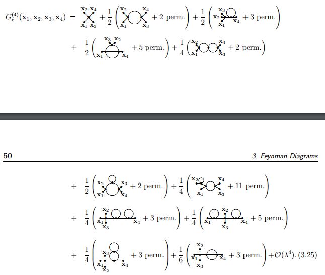
Feynman Diagram Expansion of the Connected Four-Point Green's Function — The Fourier transform of the connected four-point Green's function, $\tilde{G}_c^{(4)}$, is given by the sum of all connected diagrams with four external points. This image shows several diagrams contributing up to order $\lambda^3$. Notice that each external line corresponds to a propagator factor, which must be 'amputated' via the LSZ formula to get the S-matrix element.

3. The Feynman Rules for the Invariant Matrix Element $M$

We are now ready to take the final step. The LSZ formula connects the S-matrix element to the Green's function:

⟨ p_{1} \dots p_{o u t} ∣ S - 1∣ k_{1} \dots k_{in} ⟩ \propto j \prod (p_{j}^{2} - m^{2}) i \prod (k_{i}^{2} - m^{2}) G ~^{(n)} (p_{j}, - k_{i})

On the right-hand side, $G ~^{(n)}$ is the sum of all connected Feynman diagrams calculated with the momentum-space rules we just found. Each of these diagrams has propagators for the external lines, of the form $\frac{i}{p ^{2} - m ^{2} + i ϵ}$ .

The LSZ formula tells us to multiply by $(p^{2} - m^{2})$ for each external leg and take the on-shell limit $p^{2} \to m^{2}$ . This procedure does two things:

It precisely cancels the propagator factor for each external line. This is what we call amputation.
It puts the external particles on-shell, making them real physical particles.

Factoring out the overall momentum-conserving delta function, we are left with $i M$ . This gives us our final, powerful set of rules.

The Momentum-Space Feynman Rules for $i M$ in $ϕ^{4}$ Theory:

To calculate $i M$ for a given process:

Draw all possible connected, amputated Feynman diagrams for the process up to the desired order in $λ$ .
For each internal line carrying momentum $k$ , write a factor for the propagator:
$\frac{i}{k ^{2} - m ^{2} + i ϵ}$
For each vertex, write a factor of:
$- iλ$
(The $\frac{1}{4 !}$ in the Lagrangian is precisely cancelled by the 4! ways to connect the four lines at the vertex during the Wick expansion.)
For each vertex, enforce momentum conservation. The sum of momenta flowing into the vertex must equal the sum of momenta flowing out.
Integrate over each undetermined loop momentum $k$ :
$\int \frac{d ^{4} k}{( 2 π ) ^{4}}$
Divide the whole expression by the symmetry factor of the diagram. This is an integer that corrects for overcounting due to diagram symmetries.
Sum the contributions from all diagrams.

Test your understanding!

Consider the lowest-order (tree-level) contribution to $2 \to 2$ scattering ( $ϕϕ \to ϕϕ$ ) with incoming momenta $p_{1}, p_{2}$ and outgoing momenta $p_{3}, p_{4}$ .

Draw the single amputated Feynman diagram that describes this process at order $λ$ .
Using the rules above, write down the expression for $i M$ . What is the symmetry factor?

Show answer

The diagram is just a single point (the vertex) with four lines attached: two incoming ( $p_{1}, p_{2}$ ) and two outgoing ( $p_{3}, p_{4}$ ). There are no internal lines or loops.
We apply the rules:
- There are no internal propagators.
- There is one vertex, contributing a factor of $- iλ$ .
- Momentum conservation at the vertex is automatically handled by the overall delta function $(2 π)^{4} δ^{(4)} (p_{1} + p_{2} - p_{3} - p_{4})$ which we have factored out of $M$ .
- There are no loops to integrate over.
- The diagram has no symmetries that would lead to overcounting in the Wick expansion, so the symmetry factor is 1.
Therefore, the result is simply:
$i M = - iλ$
This gives $M = - λ$ . It's that simple!

Conclusion

Today, we have distilled the entire machinery of perturbative QFT into a practical and elegant algorithm. By combining the Dyson series, Wick's theorem, and the physical insight of the LSZ formula, we have derived the momentum-space Feynman rules. These rules provide a direct method to calculate the invariant matrix element $M$ , which is the heart of any scattering calculation.

Key Takeaways:

The perturbative expansion of correlation functions can be represented by Feynman diagrams, where lines are propagators and junctions are interaction vertices.
Integrating over vertex positions in position space leads to momentum conservation at each vertex in momentum space.
The LSZ formula provides the physical justification for amputating the external legs of the Green's function diagrams to obtain the S-matrix element.
The final Feynman rules for $M$ are a simple prescription for translating a diagram into a mathematical expression for the scattering amplitude.

Preview of the Next Lesson:

We've derived the rules and even used them for a trivial case. In the next lesson, we will put them to work on a more interesting problem: we will calculate the full tree-level $2 \to 2$ scattering amplitude in $ϕ^{4}$ theory, which involves more than one diagram. This will be our first complete calculation of a QFT scattering process.

Recommended resources

1. From Perturbation Theory to Position-Space Diagrams

2. Translating to Momentum Space

3. The Feynman Rules for the Invariant Matrix Element M

Conclusion

3. The Feynman Rules for the Invariant Matrix Element $M$