Monte Carlo Event Generation for 2→2 Scalar Scattering

1. From Cross-Sections to Event Generation

So far, we have focused on the differential cross-section $d\sigma /d\Omega$. This function can be interpreted as a probability distribution: it tells us the relative probability of particles scattering into a given solid angle $d\Omega$.

An event generator's job is to act like a virtual particle accelerator. It "collides" particles and generates final states (in our case, the scattering angles $\theta$ and $\varphi$) according to this probability distribution. By generating millions of such "events," we can build up statistical distributions of observables (like the scattering angle) that can be directly compared to histograms measured in a real detector.

The core of this process is a numerical technique known as the Monte Carlo method, which uses random sampling to solve problems that might be difficult to handle analytically.

2. The Accept-Reject Method

How do we generate random numbers that follow a specific, non-uniform probability distribution? One of the simplest and most elegant Monte Carlo techniques is the accept-reject method.

Imagine you want to generate random points under a complicated curve $f(x)$. The accept-reject algorithm works as follows:

1. Enclose your function $f(x)$ within a simpler shape for which you can easily generate random points (e.g., a rectangle). Let the height of this rectangle be $f_{\text{max}}$, the maximum value of $f(x)$.
2. Generate a random point $(x_{\text{trial}},y_{\text{trial}})$ uniformly within this rectangle.
3. Accept the point if $y_{\text{trial}}<f(x_{\text{trial}})$. This means the point falls under the curve.
4. Reject the point if it's above the curve.
5. The $x$-coordinates of the accepted points will be distributed according to the probability distribution defined by $f(x)$.

This "hit-or-miss" approach is a cornerstone of Monte Carlo simulation.

3. Application to ${\varphi }^4$ Scattering

Let's apply this to our $2\to 2$ scattering process. The probability of scattering into a solid angle element $d\Omega =\sin \theta d\theta d\varphi$ is proportional to $d\sigma /d\Omega$. Therefore, the probability distribution for the angles $(\theta ,\varphi )$ is:

For our ${\varphi }^4$ theory, $d\sigma /d\Omega =\frac{{\lambda }^2}{128{\pi }^{2}s}$, which is a constant. So, the probability distribution simplifies to:

This means the distribution is uniform in $\varphi$ (from 0 to $2\pi$) but depends on $\theta$ (from 0 to $\pi$). Our task is to generate pairs of $(\theta ,\varphi )$ that follow this distribution.

Algorithm:

1. Generate $\varphi$: Since the distribution is uniform in $\varphi$, we can generate it directly: $\varphi =2\pi \times \text{rand}$, where $\text{rand}$ is a uniform random number in $[0,1]$.
2. Generate $\theta$: The probability distribution for $\theta$ is $P(\theta )\propto \sin \theta$. We will use the accept-reject method.
   • The function we want to sample from is $f(\theta )=\sin \theta$. Its domain is $[0,\pi ]$.
   • The maximum value is $f_{\text{max}}=\sin (\pi /2)=1$.
   • Trial Generation:
     a. Generate a trial angle ${\theta }_{\text{trial}}$ uniformly from $[0,\pi ]$.
     b. Generate a second uniform random number $u$ from $[0,1]$.
   • Accept-Reject Step:
     c. If $u\le \sin ({\theta }_{\text{trial}})$, we accept ${\theta }_{\text{trial}}$.
     d. Otherwise, we reject it and try again with a new ${\theta }_{\text{trial}}$ and $u$.

The set of accepted $(\theta ,\varphi )$ pairs are our generated "events."

4. Advanced Topic: Variance Reduction

The simple accept-reject method is powerful, but it can be inefficient if the function you are sampling has very sharp peaks, leading to a low acceptance rate. More advanced techniques, like importance sampling, are used to improve efficiency. The idea is to use a trial distribution that more closely matches the shape of the true distribution, concentrating the sampling effort in the "important" regions.

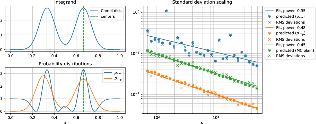
While we won't implement these advanced methods today, it's important to know they exist, as they are fundamental to professional-grade event generators like PYTHIA and Herwig.

5. Your Task: Build a Simple Event Generator

Now, let's put this into practice. Your task is to write a Python script that implements the accept-reject algorithm to generate events for ${\varphi }^4$ scattering and visualize the results.

Instructions:

1. Set up your script: You will need numpy for random number generation and mathematical functions, and matplotlib.pyplot for plotting.
2. Set the number of events: Define a variable, e.g., num_events = 10000, for the number of accepted events you want to generate.
3. Implement the generation loop:
   • Create an empty list to store your accepted $\theta$ and $\varphi$ angles.
   • Start a while loop that continues until you have collected num_events.
   • Inside the loop, perform one step of the accept-reject algorithm for $\theta$ described in Section 3.
   • If an angle is accepted, generate a corresponding uniform $\varphi$ and append both to your list of events.
4. Analyze the results:
   • Once the loop finishes, you will have a list of events.
   • Convert your list of $\theta$ angles to a NumPy array and calculate $\cos \theta$.
   • Use matplotlib.pyplot.hist to create two histograms:
     a. One for the distribution of the generated $\theta$ angles.
     b. One for the distribution of the generated $\cos \theta$ values.
5. Interpret the plots:
   • Does the histogram for $\theta$ resemble a $\sin \theta$ curve?
   • Is the histogram for $\cos \theta$ approximately flat, as predicted?

This exercise provides a hands-on feel for how theoretical distributions are turned into simulated data. For a real-world application of these very techniques, the paper "Particle physics phenomenology with python 3" (resource LINK) demonstrates using Monte Carlo integration to calculate cross-sections for a process in Fermi theory, and importantly, provides their Python code on GitHub—a great example of these principles in practice.

Conclusion

Congratulations! You have now built a rudimentary, but conceptually complete, Monte Carlo event generator. You've gone beyond calculating a single number and have simulated the statistical distribution of scattering outcomes predicted by a quantum field theory.

Key Takeaways:

• An event generator uses Monte Carlo methods to produce samples of final-state particle configurations (e.g., momenta, angles) according to the probability distribution predicted by a given theory ($|\mathcal{M}{|}^2$).
• The accept-reject method is a fundamental algorithm for sampling from an arbitrary probability distribution by generating trial events from a simpler distribution and stochastically accepting or rejecting them.
• For isotropic scattering (like in our simple ${\varphi }^4$ theory), the distribution of scattering events is uniform in the azimuthal angle $\varphi$ and in $\cos \theta$.

This lesson concludes our first deep dive into a specific model, the ${\varphi }^4$ theory. You have derived its Feynman rules, calculated a tree-level scattering amplitude, computed the cross-section, and now built a tool to simulate the events themselves.

Preview of the Next Lesson:
So far, we have only dealt with spin-0 scalar particles. The real world, however, is dominated by spin-1/2 fermions (electrons, quarks) and spin-1 bosons (photons, gluons). In the next module, we will begin our study of fermions by deriving the cornerstone of relativistic quantum mechanics: the Dirac equation. This will open the door to describing electrons and, eventually, to the theory of Quantum Electrodynamics (QED).