Operators and Zero-Point Energy

Hello! Welcome to your sixth lesson on Quantum Field Theory.

In our last lesson, we constructed the stage and the actors for our theory. We defined the vacuum state $∣0 ⟩$ as the ground state of the field and saw how applying creation operators $a^_{p}^{†}$ populates this vacuum with particles, building up the entire Hilbert space known as Fock space.

Today, we will bring dynamics into the picture by deriving the operators for the total energy and momentum of the field. This lesson directly addresses the learning outcome: to calculate the Hamiltonian and momentum operators in terms of creation and annihilation operators, identifying the zero-point energy. This is a cornerstone calculation that reveals a famous and deep feature of quantum fields: the infinite energy of empty space.

1. The Hamiltonian of the Scalar Field

Our starting point is the classical Hamiltonian for the Klein-Gordon field, which you'll recall from our earlier lessons on Noether's theorem. It is the spatial integral of the Hamiltonian density $H$ :

H = \int d^{3} x H = \int d^{3} x \frac{1}{2} (π^{2} (x) + (\nabla ϕ (x))^{2} + m^{2} ϕ^{2} (x))

To quantize this, we promote the fields $ϕ (x)$ and $π (x)$ to the Heisenberg picture operators $ϕ^(x)$ and $π^(x)$ that we've been working with. Our goal is to re-express the Hamiltonian operator $H^$ in terms of the creation and annihilation operators $a^_{p}^{†}$ and $a^_{p}$ , which have a clearer physical interpretation in the context of Fock space.

The process involves substituting the Fourier expansions for $ϕ^(x)$ and $π^(x)$ into the expression for $H^$ . The calculation is algebraically intensive but methodologically straightforward. Here is a sketch of the main steps:

Substitution: Replace $ϕ^$ and $π^$ with their integral representations involving $a^_{p}$ and $a^_{p}^{†}$ . This results in an expression with an integral over $d^{3} x$ and, for each squared term, two momentum integrals (e.g., over $d^{3} p$ and $d^{3} q$ ).
Spatial Integration: The key step is to perform the integral over space. The terms will involve exponentials like $e^{i (p + q) \cdot x}$ . The spatial integral $\int d^{3} x e^{i (p + q) \cdot x}$ yields a Dirac delta function, $(2 π)^{3} δ^{(3)} (p + q)$ .
Momentum Integration: This delta function is then used to eliminate one of the momentum integrals, enforcing the condition $q = - p$ .
Simplification: The remaining expression is a single integral over $p$ . After significant algebraic simplification, using facts like $ω_{p} = ω_{- p}$ , we arrive at the result.

This derivation is a classic rite of passage in QFT. The following video provides an extremely detailed, step-by-step walkthrough of the entire calculation. Given your preference for detailed derivations, following this will be very insightful.

Quantizing the Klein-Gordon Field as Harmonic Oscillators - FULLY EXPLAINED!

The calculation to get the Hamiltonian is quite involved. This video provides a very detailed, step-by-step derivation, leaving no algebraic stone unturned. It's an excellent way to see exactly how the field expansions are substituted and simplified.

Watch the segment from 1:06:19 to 1:23:55. Follow the substitution of the field operators into the Hamiltonian density, the integration over space to get the delta function, and the subsequent algebraic simplification to arrive at the final form of the Hamiltonian in terms of the ladder operators. Don't worry about memorizing every step, but focus on the logic of the procedure.

After the dust settles, the Hamiltonian takes the form:

H^= \int \frac{d ^{3} p}{( 2 π ) ^{3}} \frac{ω _{p}}{2} (a^_{p}^{†} a^_{p} + a^_{p} a^_{p}^{†})

where $ω_{p} = ∣ p ∣^{2} + m^{2}$ is the energy of a single particle with momentum $p$ . This expression is beautifully suggestive; it looks like a sum over the Hamiltonians of all the harmonic oscillator modes of the field.

2. The Problem of Zero-Point Energy

Let's look more closely at the expression for $H^$ . Using the commutation relation $[a^_{p}, a^_{q}^{†}] = (2 π)^{3} δ^{(3)} (p - q)$ , we can reorder the second term:

a^_{p} a^_{p}^{†} = a^_{p}^{†} a^_{p} + (2 π)^{3} δ^{(3)} (0)

Substituting this back into the Hamiltonian gives:

H^= \int \frac{d ^{3} p}{( 2 π ) ^{3}} ω_{p} a^_{p}^{†} a^_{p} + \int \frac{d ^{3} p}{( 2 π ) ^{3}} \frac{ω _{p}}{2} (2 π)^{3} δ^{(3)} (0)

The first term is an operator that, as we'll see, counts the energy of particles present in a state. The second term is a constant—a c-number, not an operator. This constant is the energy of the vacuum state, $E_{0} = ⟨ 0∣ H^∣0 ⟩$ , also known as the zero-point energy.

And it's infinite.

This infinity comes from two sources:

The $δ^{(3)} (0)$ term: Formally, $δ^{(3)} (x) = \int \frac{d ^{3} k}{( 2 π ) ^{3}} e^{i k \cdot x}$ , so $δ^{(3)} (0) = \int \frac{d ^{3} k}{( 2 π ) ^{3}} = \frac{V}{( 2 π ) ^{3}}$ , where $V$ is the volume of space. This is an infrared (IR) divergence, arising because we are considering an infinite volume. We can think of the problem in terms of energy density, which removes this factor.
The $\int d^{3} p ω_{p}$ integral: Even for the energy density, we have an integral $\int d^{3} p ∣ p ∣^{2} + m^{2}$ which diverges as $∣ p ∣ \to \infty$ . This is an ultraviolet (UV) divergence, arising from the contribution of an infinite number of modes with arbitrarily high momentum.

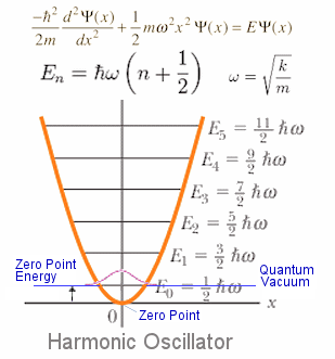
This is a direct consequence of treating the field as an infinite collection of quantum harmonic oscillators. Each oscillator has a ground state energy of $\frac{1}{2} ℏ ω$ . The total vacuum energy is the sum over all of these.

Quantum Harmonic Oscillator Energy Levels and Zero-Point Energy — This diagram illustrates the quantized energy levels of a single harmonic oscillator. The lowest possible energy is the zero-point energy, $E_0 = \frac{1}{2}\hbar\omega$. The infinite zero-point energy of the quantum field is the sum of these ground state energies over all possible momentum modes.

3. Renormalization and Normal Ordering

How do we handle this infinite vacuum energy? The key physical insight is that, in the absence of gravity, we can only ever measure energy differences, not absolute energy. The infinite energy of the vacuum is a constant offset that affects all states equally. We can therefore "renormalize" our definition of energy by subtracting this constant, effectively setting the vacuum energy to zero.

The formal procedure to achieve this is called normal ordering. We define the normal-ordered product of a string of operators, denoted by colons : \dots :, as the expression with all creation operators moved to the left of all annihilation operators. For our purposes, this simply means:

: a^_{p} a^_{q}^{†} :\equiv a^_{q}^{†} a^_{p}

When we apply normal ordering to our Hamiltonian, we get the physically measurable Hamiltonian:

: H^:=: \int \frac{d ^{3} p}{( 2 π ) ^{3}} \frac{ω _{p}}{2} (a^_{p}^{†} a^_{p} + a^_{p} a^_{p}^{†}) := \int \frac{d ^{3} p}{( 2 π ) ^{3}} ω_{p} a^_{p}^{†} a^_{p}

This normal-ordered Hamiltonian, by construction, gives zero when acting on the vacuum, $: H^: ∣0 ⟩ = 0$ , and gives the sum of particle energies for any other state. From now on, we will implicitly assume all our Hamiltonians (and other observables) are normal-ordered.

The following reading provides a concise and clear discussion of this crucial concept.

Quantum Field Theory

Now that we've derived the Hamiltonian, let's look closer at the zero-point energy and the standard method for dealing with it. This section from the QFT notes by Rumsey, et al., provides a very clear explanation.

Read the subsection 'Energy of the vacuum state and renormalisation' (starts on page 19). It begins right after the expressions for the Hamiltonian and momentum operators. Pay close attention to the calculation of the vacuum energy in Eq. (127), the reasoning for its divergence, and the introduction of the normal-ordered Hamiltonian in Eq. (135) as the solution.

4. The Momentum Operator

A completely analogous calculation can be performed for the total momentum operator of the field, $P^$ . Starting from the conserved Noether current $T^{0 i} = \partial^{0} ϕ \partial^{i} ϕ = - π \nabla_{i} ϕ$ , the momentum operator is:

P^= - \int d^{3} x π^(x) \nabla ϕ^(x)

Following the same procedure of substitution and integration, and applying normal ordering, we arrive at a beautifully simple result:

: P^:= \int \frac{d ^{3} p}{( 2 π ) ^{3}} p a^_{p}^{†} a^_{p}

This expression has a transparent physical interpretation. The operator $N^_{p} \equiv a^_{p}^{†} a^_{p}$ acts as a number operator (density in momentum space), which counts the number of particles with momentum $p$ . Thus, the total momentum of the field is simply the sum (integral) of the momentum of each particle, $p$ , multiplied by the number of particles with that momentum.

The following video derives both the Hamiltonian and momentum operators from the more formal starting point of the energy-momentum tensor, which should connect well with your background in classical mechanics and field theory.

Quantum Field Theory I - Lecture 8

The derivation for the momentum operator follows a similar path to the Hamiltonian. This video segment derives both the Hamiltonian and the momentum operator starting from the energy-momentum tensor obtained via Noether's theorem, providing a rigorous foundation.

Watch the segment from 25:11 to 33:22. The lecturer first identifies the Hamiltonian and momentum densities from the stress-energy tensor. Focus on the derivation of the momentum operator \hat{P} starting around 29:00. See how substituting the field expansions leads to the final form in terms of creation and annihilation operators and how this confirms the particle interpretation.

Test your understanding!

Show that a one-particle state $∣ q ⟩ = a^_{q}^{†} ∣0 ⟩$ is an eigenstate of the normal-ordered Hamiltonian $: H^:$ with the correct relativistic energy $E_{q} = ω_{q}$ . Use the rescaled operators where $[a^_{p}, a^_{q}^{†}] = δ^{(3)} (p - q)$ for simplicity, which corresponds to $: H^:= \int d^{3} p ω_{p} a^_{p}^{†} a^_{p}$ .

Show answer

We want to calculate $: H^: ∣ q ⟩$ .

: H^: ∣ q ⟩ = (\int d^{3} p ω_{p} a^_{p}^{†} a^_{p}) a^_{q}^{†} ∣0 ⟩ = \int d^{3} p ω_{p} a^_{p}^{†} a^_{p} a^_{q}^{†} ∣0 ⟩

Now, we use the commutation relation to move $a^_{p}$ to the right: $a^_{p} a^_{q}^{†} = a^_{q}^{†} a^_{p} + δ^{(3)} (p - q)$ .

: H^: ∣ q ⟩ = \int d^{3} p ω_{p} a^_{p}^{†} (a^_{q}^{†} a^_{p} + δ^{(3)} (p - q)) ∣0 ⟩ = \int d^{3} p ω_{p} a^_{p}^{†} a^_{q}^{†} a^_{p} ∣0 ⟩ + \int d^{3} p ω_{p} a^_{p}^{†} δ^{(3)} (p - q) ∣0 ⟩

The first term is zero because $a^_{p} ∣0 ⟩ = 0$ for all $p$ . The second term can be simplified by using the delta function to perform the integral over $p$ :

: H^: ∣ q ⟩ = 0 + ω_{q} a^_{q}^{†} ∣0 ⟩ = ω_{q} ∣ q ⟩

This confirms that $∣ q ⟩$ is an eigenstate of the Hamiltonian with eigenvalue $ω_{q} = ∣ q ∣^{2} + m^{2}$ , the correct relativistic energy for a particle of mass $m$ and momentum $q$ .

Conclusion

This lesson has been a major step in connecting the formal machinery of canonical quantization to the physical world of particles. By expressing the fundamental observables of energy and momentum in terms of creation and annihilation operators, we have solidified the particle interpretation of the field's excitations.

Key Takeaways:

The Hamiltonian and momentum operators for the free scalar field can be expressed as integrals over creation and annihilation operators.
The raw Hamiltonian contains an infinite constant term, the zero-point energy, which is the sum of ground-state energies of all the field's harmonic oscillator modes.
This infinity is handled by normal ordering, a procedure that redefines the zero of energy to be the vacuum energy, yielding a physically meaningful operator that measures the energy of particles above the vacuum.
The normal-ordered Hamiltonian and momentum operators are:
$: H^:= \int \frac{d ^{3} p}{( 2 π ) ^{3}} ω_{p} a^_{p}^{†} a^_{p} and : P^:= \int \frac{d ^{3} p}{( 2 π ) ^{3}} p a^_{p}^{†} a^_{p}$
These operators simply sum the energy and momentum of all particles present in a given state.

Preview of the Next Lesson:

So far, we have a "static" picture of our field theory—we can describe states with a fixed number of non-interacting particles. The next crucial concept is to understand how particles propagate from one point to another. In the next lesson, we will derive the Feynman propagator for the scalar field as the vacuum expectation value of a time-ordered product of fields. The propagator is the central object that will allow us to describe interactions and calculate scattering processes later on.

Recommended resources

1. The Hamiltonian of the Scalar Field

2. The Problem of Zero-Point Energy

3. Renormalization and Normal Ordering

4. The Momentum Operator

Conclusion