Wilson Loop Expectation Value Calculation

1. What is a Wilson Loop?

In the continuum, a Wilson loop is defined as the path-ordered exponential of the gauge field integrated around a closed loop $C$:
$W(C)=\text{Tr}\left(\mathcal{P}\exp \left(ig{\oint }_C{A}_{\mu }(x)d{x}^{\mu }\right)\right)$
The trace ensures gauge invariance. On the lattice, this intimidating expression simplifies beautifully. Recall that the link variable $U_{\mu }(x)$ acts as a "parallel transporter" from site $x$ to $x+\hat{\mu }$. A Wilson loop is then simply the product of the link variables along a closed path on the lattice.

For a closed loop $C$ composed of a sequence of links $(x_1,{\mu }_1),(x_2,{\mu }_2),\dots ,(x_L,{\mu }_L)$, the Wilson loop is:
$W(C)=\text{Tr}\left(U_{{\mu }_L}(x_L)\cdots U_{{\mu }_2}(x_2)U_{{\mu }_1}(x_1)\right)$

The ordering of the matrix multiplication is crucial and follows the direction of the path. For the U(1) gauge group we are studying, the link variables are complex numbers (1x1 matrices), so they commute, the trace is trivial, and path-ordering is not an issue. The Wilson loop is simply the product of the complex numbers along the path.

2. From Path Integrals to Monte Carlo Averages

The vacuum expectation value (VEV) of an observable $\mathcal{O}$ in quantum field theory is given by the path integral:
$⟨\mathcal{O}⟩=\frac{1}{Z}\int \mathcal{D}U\mathcal{O}[U]e^{-S[U]}$
where $Z=\int \mathcal{D}U{e}^{-S[U]}$ is the partition function.

The power of our Monte Carlo simulation lies in its ability to evaluate this high-dimensional integral numerically. The Metropolis algorithm you implemented generates a sequence of $N_{\text{meas}}$ configurations $\{U^{(i)}\}$ that are sampled directly from the probability distribution $P[U]=\frac{1}{Z}{e}^{-S[U]}$. This process, known as importance sampling, transforms the path integral from a complex integration problem into a simple arithmetic average.

For a Wilson loop $W(C)$, the expectation value is approximated by the average of $W(C)$ over your generated ensemble:
$⟨W(C)⟩\approx \frac{1}{N_{\text{meas}}}{\sum }_{i=1}^{N_{\text{meas}}}W(C)[U^{(i)}]$
Here, $W(C)[U^{(i)}]$ is the value of the Wilson loop calculated on the $i$-th gauge field configuration.

3. Practical Calculation of Wilson Loops

Now, let's outline the concrete steps to compute the expectation value of an $R\times T$ rectangular Wilson loop. Given your experience with simulations on grids, the logic should be quite familiar.

Let's say we want to compute the average of a rectangular loop of size $R\times T$ lying in the $\mu -\nu$ plane.

Step 1: Compute the loop on a single configuration

To improve our statistics for a single configuration, we should average the loop over all possible starting positions $n$ and all non-equivalent plane orientations $(\mu ,\nu )$.

The value of a single $R\times T$ loop starting at site $n$ in the $\mu -\nu$ plane is the product of $2R+2T$ link variables. For example, for a $2\times 1$ loop in the $x-t$ plane ($\mu =0,\nu =1$):
$W_{2\times 1}(n)=U_0(n)U_0(n+\hat{x})U_1(n+2\hat{x})U_0^{†}(n+\hat{x}+\hat{t})U_0^{†}(n+\hat{t})U_1^{†}(n)$
Note the use of the conjugate (inverse) links for paths in the negative direction. Your computational task is to implement this product. You can do this by creating shifted copies of your link arrays, which is an efficient vector operation.

Step 2: Average over the entire lattice

The expectation value for a single configuration, $⟨W_{R\times T}{⟩}_{\text{config}}$, is the average over all starting sites n, and typically, all plane orientations.

where $V$ is the number of lattice sites. We take the real part, consistent with how we defined the plaquette's contribution to the Wilson action.

Step 3: Average over the ensemble

Finally, the full VEV is the average of these single-configuration values over your entire ensemble of N_meas thermalized, decorrelated configurations.

# Pseudocode for the measurement process
# Assume you have a list of configurations: `ensemble = [U1, U2, ...]`

total_loop_average = 0.0
for U_config in ensemble:
    # Average W(R,T) over all starting sites n for this one config
    config_average = average_loop_over_lattice(U_config, R, T)
    total_loop_average += config_average

final_vev = total_loop_average / len(ensemble)

4. Physical Motivation: Probing Confinement

Why go to all this trouble? The behavior of Wilson loops as their area increases is a direct probe of confinement. For a rectangular loop of spatial size $R$ and temporal extent $T$, its expectation value for large $T$ is related to the potential energy $V(R)$ between a static quark-antiquark pair separated by distance $R$:
$⟨W(R,T)⟩\sim e^{-V(R)T}$

This relationship gives us two famous criteria:

1. Area Law: If $⟨W(R,T)⟩\sim e^{-\sigma RT}$ (decays with the area), it implies a linearly rising potential $V(R)=\sigma R$. This is the signature of confinement. The force between the quarks is constant, and it would take infinite energy to separate them.
2. Perimeter Law: If $⟨W(R,T)⟩\sim e^{-c(R+T)}$ (decays with the perimeter), the potential $V(R)$ flattens to a constant at large distances. The theory is not confining, and the particles can be separated. This is the behavior seen in QED (a Coulomb phase).

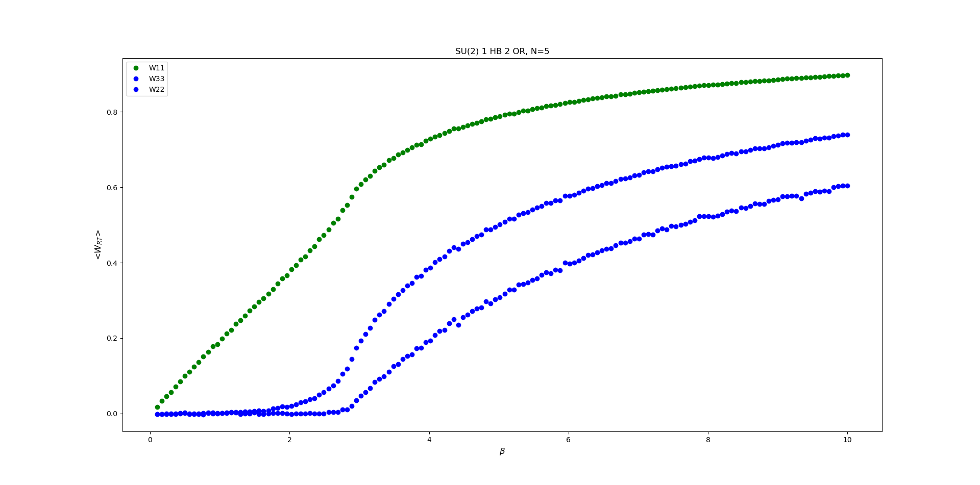
By calculating $⟨W(R,T)⟩$ for various $R$ and $T$, we can determine which regime our simulated theory is in.

Conclusion

Today, we have connected the output of our Monte Carlo simulation to a physically meaningful, gauge-invariant observable. You have learned how to define a Wilson loop on the lattice and, crucially, how to calculate its expectation value as an average over your generated configurations.

Key Takeaways:

• A Wilson loop is the trace of a path-ordered product of link variables along a closed loop. It is the lattice version of a fundamental gauge-invariant operator.
• The expectation value of a Wilson loop, defined as a path integral, can be numerically computed by averaging its value over an ensemble of configurations generated by a Monte Carlo algorithm.
• The calculation involves three averaging steps: over loop orientations, over starting positions on the lattice, and finally, over the entire ensemble of configurations.
• The physical motivation for this calculation is profound: the area-law or perimeter-law behavior of large Wilson loops reveals whether the underlying theory is confining.

Preview of the Next Lesson:

We have laid all the groundwork. We know what a Wilson loop is and how to calculate its expectation value. In the next lesson, we will focus entirely on the physical interpretation. We will relate the area law behavior of Wilson loops to the static quark-antiquark potential and the concept of confinement. You will learn how to extract the string tension $\sigma$ from your data, which is a quantitative measure of the confining force.