Introduction
Welcome to your next lesson on perfect competition. In our previous session, we established the core characteristics of a perfectly competitive market. The most crucial takeaway was that firms in this environment are price takers. This means they face a perfectly horizontal demand curve, and as a result, the market price is equal to their marginal revenue (P = MR).
Today, we will build directly on that foundation. The learning outcome for this lesson is to determine the short-run profit-maximizing output and shutdown decision for a perfectly competitive firm. We'll break this down into a two-step process:
- First, we'll use the universal profit-maximization rule (MR = MC) to find the ideal quantity of output for the firm.
- Second, we'll analyze the firm's costs at that output level to decide if it should make a profit, operate at a loss, or shut down entirely in the short run.
This lesson combines graphical analysis with clear decision rules, providing the practical framework you'll need for the CFA exam.
1. The Profit-Maximizing Output: Where Price Equals Marginal Cost
Every profit-maximizing firm, regardless of market structure, should produce up to the point where the revenue from the last unit sold equals the cost of producing it. This is the MR = MC rule. If MR > MC, the firm can increase profit by producing more. If MR < MC, it's producing too much and should cut back.
In our last lesson, we saw that for a perfectly competitive firm, P = MR. By substituting Price for Marginal Revenue, we arrive at the specific rule for a perfectly competitive firm:
Profit is maximized at the quantity (Q) where P = MC.
One technical detail is that this rule applies where the marginal cost curve is rising. If P = MC where the MC curve is falling, producing more would mean MC falls further below P, increasing profit, so that cannot be the profit-maximizing point.
To see this principle in action, let's watch a short video.
Maximizing Profit and the Shut Down Rule- Micro Topics 3.5 and 3.6
The following clip from Jacob Clifford clearly explains the logic behind the MR = MC rule and shows how to find the profit-maximizing quantity on a graph.
Watch the segment from 00:40 to 02:06. Focus on the core argument: why you always produce where MR = MC and why you stop at that point.
As the video demonstrates, finding this quantity is the first and most critical step. You locate the market price on the vertical axis, trace across to where it intersects the marginal cost (MC) curve, and drop down to the horizontal axis to find the profit-maximizing quantity, Q*.
2. Is the Firm Making a Profit or a Loss?
Once we've found the optimal quantity (Q*), the next question is: is the firm actually profitable at this output level? The answer depends on the relationship between the price and the Average Total Cost (ATC) at Q*.
Remember the basic profit formula:
We can express this on a per-unit basis:
Since Price = AR for a competitive firm, this simplifies to:
This leads to three possible short-run outcomes at the profit-maximizing quantity Q*:
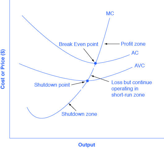
- Economic Profit: If P > ATC, the firm is earning more per unit than its average cost. It is making an economic profit.
- Zero Economic Profit (Break-Even): If P = ATC, the firm's revenue just covers all its costs, including opportunity costs. This is the break-even point. The firm is earning a normal profit but not an economic profit.
- Economic Loss: If P < ATC, the firm is not covering its average costs and is incurring an economic loss.
The following video segment illustrates these three scenarios.
Maximizing Profit and the Shut Down Rule- Micro Topics 3.5 and 3.6
Continuing with the same video, this part shows how to use the ATC curve to determine whether the firm is making a profit, a loss, or breaking even.
Watch from 02:06 to 03:03. Notice how the MR = MC rule determines the quantity, but the position of the ATC curve at that quantity determines the profit or loss.
This brings us to a crucial decision. If a firm is making a loss, should it just stop producing?
3. The Short-Run Shutdown Decision
In the short run, a firm has both fixed costs (like rent) and variable costs (like labor and materials). Fixed costs must be paid even if the firm produces zero output. Therefore, when facing a loss, the firm has two options:
- Shut down temporarily: Produce nothing (Q=0) and incur a loss equal to its Total Fixed Costs (TFC).
- Continue to produce: Produce at Q* (where P=MC) and incur a loss.
The logical choice is the one that results in a smaller loss. The decision hinges on whether the revenue generated can cover the variable costs of production.
This gives us the shutdown rule:
- If P ≥ Average Variable Cost (AVC), the firm should continue to produce. Each unit sold covers its own variable cost and contributes something toward paying the fixed costs. The loss will be less than the Total Fixed Costs.
- If P < Average Variable Cost (AVC), the firm should shut down. Each unit sold fails to even cover its own variable cost. Continuing to produce would add to the losses on top of the fixed costs.
The shutdown point is the price and quantity where the firm is indifferent between operating and shutting down. This occurs at the minimum point of the AVC curve, where P = min(AVC).
The "inverted stoplight" analogy in the next video provides an excellent mental model for this entire decision process.
Maximizing Profit and the Shut Down Rule- Micro Topics 3.5 and 3.6
This clip masterfully explains the shutdown rule using a simple 'stoplight' analogy that connects price to the ATC and AVC curves.
Watch from 03:03 to 05:50. Pay close attention to the three zones: green (profit), yellow (loss, but operate), and red (shutdown). Understand why it makes sense to operate at a loss in the 'yellow' zone.
The following graph consolidates all these rules into a single visual.
To solidify these concepts, let's turn to a CFA-focused reading that summarizes these rules and provides a practical example.
Breakeven Analysis Explained | CFA Level 1 - AnalystPrep
This article from AnalystPrep explains the breakeven and shutdown analysis in a way that is directly relevant to the CFA exam. Focus on the decision rules and the summary table.
Read the sections 'Shutdown Analysis', 'Example: Shut-down Point of Production', and the practice question #2. Pay special attention to the table that outlines the short-run and long-run decisions based on revenue and costs. Work through the numerical example to see the logic applied.
The table in this reading is a high-yield summary that is very useful for exam review. The distinction between the short-run decision (continue vs. shut down) and the long-run decision (remain vs. leave the market) is critical.
4. A Step-by-Step Numerical Example
Let's walk through a complete problem to tie everything together. Given your mathematical background, applying these rules with concrete numbers will help cement your understanding.
Consider a firm with the following cost structure, facing a market price of $28.
| Q | P | TFC | TVC |
|---|---|---|---|
| 0 | $28 | $20 | $0 |
| 1 | $28 | $20 | $20 |
| 2 | $28 | $20 | $25 |
| 3 | $28 | $20 | $35 |
| 4 | $28 | $20 | $52 |
| 5 | $28 | $20 | $80 |
Step 1: Calculate all cost and revenue columns.
First, we compute Total Cost (TC), Average Variable Cost (AVC), Average Total Cost (ATC), Marginal Cost (MC), Total Revenue (TR), and Profit.
| Q | P | TFC | TVC | TC | AVC | ATC | MC | TR | Profit |
|---|---|---|---|---|---|---|---|---|---|
| 0 | $28 | $20 | $0 | $20 | - | - | - | $0 | -$20 |
| 1 | $28 | $20 | $20 | $40 | $20.00 | $40.00 | $20 | $28 | -$12 |
| 2 | $28 | $20 | $25 | $45 | $12.50 | $22.50 | $5 | $56 | $11 |
| 3 | $28 | $20 | $35 | $55 | $11.67 | $18.33 | $10 | $84 | $29 |
| 4 | $28 | $20 | $52 | $72 | $13.00 | $18.00 | $17 | $112 | $40 |
| 5 | $28 | $20 | $80 | $100 | $16.00 | $20.00 | $28 | $140 | $40 |
(Note: MC is the change in TC for one additional unit. For example, MC for Q=5 is $100 - $72 = $28).
Step 2: Find the profit-maximizing quantity (P=MC).
The market price is $28. Looking at the MC column, we see that MC equals $28 at an output quantity of Q=5.
Step 3: Determine profit or loss at Q=5 (P vs. ATC).
At Q=5, the price is $28 and the ATC is $20.00. Since P > ATC, the firm is making an economic profit. The profit is ($28 - $20) * 5 = $40.
Step 4: Check the shutdown condition (P vs. AVC).
This step is only necessary if the firm were making a loss. However, for completeness, at Q=5, the price of $28 is well above the AVC of $16.00. The firm should definitely produce.
This detailed, step-by-step process is precisely what you need to master for exam questions involving tables of data. This example is adapted from the "Work It Out" feature in the resource "How Perfectly Competitive Firms Make Output Decisions," which you can use for further reference.
Conclusion
In this lesson, we have moved from identifying the characteristics of perfect competition to analyzing a firm's behavior within it. We developed a clear, rule-based framework for making short-run output and operational decisions.
Key Takeaways:
- Profit-Maximizing Quantity: A perfectly competitive firm maximizes profit by producing the quantity (Q*) where P = MC.
- Profit or Loss: At Q*, the firm's financial result is determined by comparing price to Average Total Cost (ATC):
- If P > ATC, the firm earns an economic profit.
- If P = ATC, the firm breaks even (zero economic profit).
- If P < ATC, the firm incurs an economic loss.
- Shutdown Decision: If the firm is making a loss, it must decide whether to continue producing. This decision depends on comparing price to Average Variable Cost (AVC):
- If P ≥ AVC, the firm should continue to produce to minimize its loss.
- If P < AVC, the firm should shut down, as its loss would be limited to its fixed costs.
Preview of the Next Lesson:
The short-run profits we've seen today are not sustainable. The lack of entry barriers in a perfectly competitive market means that positive economic profits act as a signal, attracting new firms. In our next lesson, we will explore the consequences of this, as we describe the long-run equilibrium in a perfectly competitive market.