Hello. Last lesson measured target benefit and off-target cost across steering strengths, while retaining per-prompt results rather than relying only on averages. This lesson uses those per-example measurements for a different intervention you have already studied: activation patching. You will estimate how much a patch changes behavior on held-out examples and attach a bootstrap confidence interval to that estimate.
The distinction matters because a striking average can come from a handful of prompts. A confidence interval helps describe how much the estimated average effect might vary if the evaluation set had contained different examples. It does not, by itself, establish that the patched activation is the mechanism the model normally uses.
Start with one effect per held-out pair
In activation patching, you run a clean input and a matched corrupted input, then replace an activation in the corrupted run with the corresponding activation from the clean run. You compare the patched run with the unpatched corrupted run, keeping the scoring rule fixed.
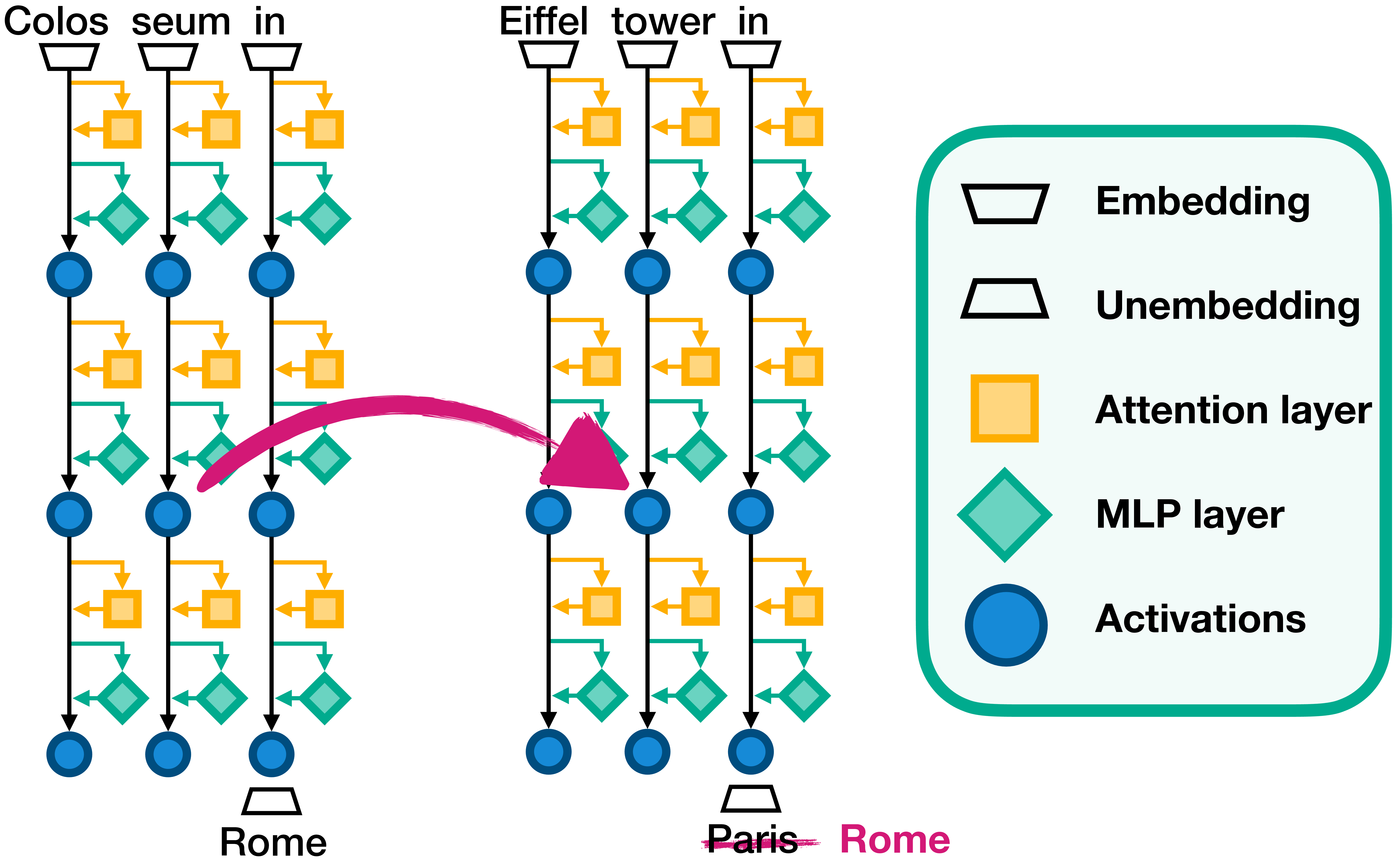
Suppose the score for held-out pair is the clean answer’s logit minus the corrupted answer’s logit. Use the same two answer tokens when scoring that pair’s corrupted and patched runs. Define its patching effect as
A positive means the patch moved this score toward the clean answer. For held-out pairs, the quantity to report is
This is a mean score change under a specified patch, not the proportion of cases fully restored to the clean answer. Those would be different statistics. State the patch site, direction of transfer, score definition, and comparison baseline alongside ; otherwise even its sign is hard to interpret.
For example, effects of and have a mean of . That number records both improvements and a deterioration, but says little about how stable the mean would be on another collection of pairs. The evaluation unit is the matched input pair, not an individual token, model run, or activation coordinate.
To build the resampling intuition, watch Bootstrapping Main Ideas!!! from StatQuest with Josh Starmer. The video uses ordinary measurements rather than patching effects; mentally substitute one measured for each observation.
StatQuest’s “Bootstrapping Main Ideas!!!” shows how repeated samples drawn from one dataset produce a distribution of estimates when repeating the whole study is impractical.
Watch replacement sampling for why a resample has the original sample size but may duplicate or omit observations. Continue through repeated estimates and the interval. Focus on the distribution of sample means, rather than interpreting its spread as variation among individual observations.
Resample the pairs, preserving the experiment
Treat the held-out pairs as the observed sample from the evaluation distribution you want to discuss. For each bootstrap replicate:
- Draw pair indices with replacement from the observed pairs.
- Compute the mean of their values.
- Save that mean.
Repeat this thousands of times. The resulting distribution approximates how the estimated mean could vary with the examples sampled. For a straightforward percentile 95% interval, take the 2.5th and 97.5th percentiles of those bootstrap means. The model does not need to be run again for every replicate: once the corrupted and patched scores are cached, resampling operates on their per-pair effects.
Preserve pairing throughout. If you resample patched scores and corrupted scores independently, a patched score from one prompt can be compared with a corrupted score from another. That simulates a different experiment and loses the advantage of comparing each prompt against its own baseline. Resampling the precomputed values is safe; resampling two score arrays using the same indices is equivalent.
Read the relevant parts of SciPy’s bootstrap documentation before implementing this. Its paired option makes the resampling unit explicit.
bootstrap — SciPy v1.17.0 Manual
Read SciPy’s documentation for the resampling procedure and the arguments used below. You need its paired-sample behavior, not every interval method or example on the page.
On the “bootstrap” page, begin just below the function signature with the three steps. Under “Parameters,” find paired and read the pairing rule; also check n_resamples, confidence_level, method, and rng. Under “Returns,” locate confidence_interval and bootstrap_distribution so you can inspect both the reported bounds and the resampled estimates.
SciPy offers several interval methods. The code below deliberately chooses method="percentile" so its bounds correspond directly to the quantiles just described; SciPy’s default is BCa, a different interval construction. Report which method you use rather than treating all “bootstrap 95% intervals” as interchangeable.
Compute an interval from cached patching runs
Assume your held-out evaluation has produced corrupt_logits and patched_logits, each shaped [N, vocab_size]. desired_ids and alternative_ids contain the two answer-token IDs for each pair. This follows the earlier patching experiment: the clean activation was obtained using the designated reference input, inserted at a fixed site in its matched corrupted input, and both resulting logits were cached.
The code makes a per-pair logit margin, then asks SciPy to resample corresponding patched and corrupted scores together.
import numpy as np
import torch
from scipy.stats import bootstrap

# One row per held-out matched pair. All four tensors are aligned.
n = corrupt_logits.shape[0]
assert patched_logits.shape == corrupt_logits.shape
assert desired_ids.shape == alternative_ids.shape == (n,)
assert n > 1

rows = torch.arange(n, device=corrupt_logits.device)
desired = desired_ids.to(corrupt_logits.device)
alternative = alternative_ids.to(corrupt_logits.device)

def margins(logits):
    return logits[rows, desired] - logits[rows, alternative]

corrupt_scores = (
    margins(corrupt_logits).detach().float().cpu().numpy()
)
patched_scores = (
    margins(patched_logits).detach().float().cpu().numpy()
)

effects = patched_scores - corrupt_scores
assert np.all(np.isfinite(effects))
point_estimate = effects.mean()

def mean_paired_difference(patched, corrupted, axis=-1):
    return np.mean(patched - corrupted, axis=axis)

result = bootstrap(
    (patched_scores, corrupt_scores),
    mean_paired_difference,
    paired=True,
    vectorized=True,
    n_resamples=10_000,
    confidence_level=0.95,
    method="percentile",
    rng=np.random.default_rng(42),
)

print("Pairs:", n)
print("Mean patching effect:", point_estimate)
print(
    "95% percentile bootstrap interval:",
    result.confidence_interval.low,
    result.confidence_interval.high,
)
print("Bootstrap standard error:", result.standard_error)
The seed makes the computational resampling reproducible; it does not make the selected prompts representative. result.bootstrap_distribution holds the 10,000 resampled means, which you can inspect for skew, unusual spikes, or instability. The standard error is the standard deviation of that distribution. If the effects are all identical, an interval can collapse; that signals what is in the observed data, not a generally reliable precision guarantee.
The same calculation can be expressed more compactly by bootstrapping the one-dimensional effects array and taking its mean. Using two arrays with paired=True here exposes the crucial design choice: patched and corrupted outcomes travel together into every resample.
A report need not show every bootstrap mean. It should, however, retain the per-pair effects and give the point estimate, interval bounds, sample size, statistic, interval method, and resample count. A result might be stated as: “Across held-out matched pairs, patching changed the mean clean-versus-corrupt logit margin by (95% paired percentile bootstrap interval: lower to upper).” Fill in the measured values; do not infer them from a visualization.
Interpret the interval at the right level
A 95% confidence interval is not a 95% probability that this fixed interval contains the true effect. Under suitable sampling assumptions, the procedure would cover the corresponding population quantity in approximately 95% of repeated studies. Here, that quantity is the mean patching effect for the evaluation distribution you sampled from, conditional on the fixed model, patch site, matching procedure, and scoring rule.
If an interval lies entirely above zero, the data support a positive average score change under that intervention on the tested distribution. If it crosses zero, the estimate is compatible with either sign at this resolution. Neither result proves that the activation is uniquely responsible for the model’s unmodified behavior, that every example responds positively, or that the finding extends to other prompt distributions.
Three design choices determine how credible that interpretation is:
- Independent evaluation units. Ten paraphrases of one template do not provide the same information as ten independently constructed cases. If several pairs come from one source example or template, ordinary pairwise resampling can make the interval too narrow. Resample source groups, keeping their associated pairs together, and specify whether the reported mean weights groups or individual pairs.
- A genuinely held-out set. Choosing a patch site, score, or preferred result after inspecting this same set makes the interval look more decisive than the selection process warrants. Select on construction or validation data; use the held-out pairs for the predeclared estimate. An interval for one selected effect does not account automatically for searching many sites.
- A defined scope of uncertainty. This bootstrap varies the sampled examples. It does not vary model training seeds, reference-activation choices, annotation judgments, or stochastic generation. Those require their own evaluation design if they matter to the claim.
These cautions also apply to an off-target metric from the previous lesson. If target and off-target scores are measured on different prompt sets, bootstrap each set using its appropriate evaluation units. Do not invent pairings between unrelated prompts merely to use a paired routine.
Takeaway
A bootstrap interval turns a patching result from a single average into an estimate with prompt-sampling uncertainty. First compute a consistently oriented effect for every held-out matched pair; then resample pairs with replacement, preserving the correspondence between patched and corrupted scores. Report the mean and interval together, and limit the conclusion to the model, intervention, metric, and evaluation distribution actually tested.
This closes the activation-interventions module. The next module begins with circuits: it will use candidate components and connections to develop more specific explanations of a computation, while keeping exact intervention tests separate from methods that merely help prioritize what to test.