Hello. Last lesson distinguished four possible units of explanation: neurons, activation directions, sparse-autoencoder latents, and circuits. The next step is to turn a proposed meaning for one of those units into a prediction that could fail. This matters when a feature appears to track a concept—or when an intervention seems to steer behavior—because neither observation, on its own, establishes what the model normally computes.
This lesson develops a testable claim using a toy arithmetic example. You will distinguish evidence that a feature tracks a concept from evidence that the model uses it, then specify observations that would weaken each claim. Allow about 35–45 minutes, including the selected resource passages.
Start by making “represents” precise
Suppose a candidate activation direction seems to represent a carry from the ones column during two-digit addition. “Represents carry” could mean at least two things:
- Readable information: its activation tends to distinguish additions with a ones-column carry from additions without one.
- Computational role: changing that feature, while controlling what else changes, alters how the model computes an answer that depends on the carry.
The first claim can hold without the second. A model might make carry information readable at a site yet use another pathway to produce its answer. Conversely, an intervention might change an answer because it disrupts several computations, not because it edited the proposed carry feature. State which claim is being tested rather than allowing “represents” to shift meaning after seeing the results.
The circuits essay Zoom In offers a useful example of building evidence for a feature description. Its curve-detector discussion moves beyond appealing visualizations to predictions about responses to varied stimuli and proposed downstream uses.
Zoom In: An Introduction to Circuits - Distill.pub
Read the curve-detector arguments in Distill’s circuits essay to see how a semantic label becomes a set of distinct empirical claims.
In “Example 1: Curve Detectors,” begin at the paragraph introducing seven arguments. Read the seven arguments, through the paragraph assessing what they establish. Focus on the difference between generating an input that activates a unit, testing its responses on varied examples, and claiming that downstream components use it.
Feature visualization can show that an input pattern causes a unit to activate. It does not, by itself, show that the unit causes a particular output. Likewise, a gallery of top-activating examples is a way to form the label “carry feature,” not a decisive test of that label: those examples were selected because they activate the feature. A stronger prediction concerns examples chosen independently of the feature score.
Write a prediction that has a place, population, and failure condition
Assume a frozen addition model is prompted to return the tens digit of a two-digit sum. The tens digits of its operands are held fixed in the following pairs:
| No ones-column carry | Ones-column carry |
|---|---|
In each pair, changing one ones digit crosses the carry threshold. The correct tens digit changes from to . These examples are a starting point, not a sufficient test set: a feature could respond to a particular digit, operand position, or prompt template instead of carry.
Here is a precise readability claim:
At a specified layer and token position, the score of a specified direction is higher for ones-column-carry inputs than for no-carry inputs on held-out, correctly solved two-digit additions across varied operand digits and prompt formats.
Let be the activation at that site for input , and let the candidate direction be . Its score is . For each matched pair , the prediction is
Before testing, specify the layer, position, direction, input population, and how consistently this inequality must hold. For example, “at least 80% of held-out matched pairs” is a possible predeclared criterion, not a universal standard. Set it using a separate development set, then leave the test pairs untouched.
The claim faces meaningful counterexamples. A direction that fires whenever it sees a should also fire for , where there is no carry. A direction that fires for large totals in the ones column might distinguish some pairs but fail on others near the threshold. Varied negative examples and neighboring cases help expose those narrower explanations. If the score fails to distinguish carry after those variations, the specified readability claim is weakened; renaming the feature to fit the test failures does not rescue the original claim.
Atticus Geiger’s lecture uses a carry variable to illustrate a more demanding standard: an internal state can be compared with a variable in a proposed causal computation, not merely assigned a label from examples.
Causal Mechanistic Interpretability (Stanford lecture 1) - Atticus Geiger
Watch “Causal Mechanistic Interpretability (Stanford lecture 1)” by Atticus Geiger for the carry-the-one example of turning a proposed internal variable into a counterfactual prediction.
Watch the carry example. Follow how the proposed high-level arithmetic variable determines what should happen when the corresponding neural state is intervened on. The key idea is to predict the changed answer before inspecting the intervened model’s output.
Add a behavioral prediction without overstating the intervention
If the stronger claim is that the model uses this feature as a carry signal, predict an output change as well. For this toy task, define the target measure as the logit margin
For a well-performing model, that margin should favor on the no-carry examples and on the carry examples. Now consider a targeted intervention at the nominated site: insert the candidate feature’s value from a carry example into a matched no-carry run, while leaving other activation information as unchanged as the method permits. The predicted effect is an increase in . In the reverse intervention, the predicted effect is a decrease in .
This is more informative than predicting “the answer will change.” It says which way a specified measure should move under each intervention direction. It also separates the proposed carry signal from generic damage: an edit that merely makes both answers less likely or produces incoherent output has not demonstrated the predicted computation.
The choice of what to replace matters. Replacing an entire activation vector from into a run on transfers every difference encoded at that site, not only carry. A successful whole-vector patch can implicate the site in the difference between these inputs; it cannot, by itself, establish that the nominated direction carries the effect. A more targeted edit and controls for unrelated changes are needed for that narrower claim.
Read a short introduction to patching, then its guidance on prompt choice:
How to use and interpret activation patching
Read these passages from “How to use and interpret activation patching” to connect the predicted output change with an actual intervention design—and to see why the chosen input pair determines what can be concluded.
In Section 1.2, “How is this related to ablation?”, begin with the distinction between zeroing and replacing activations. Continue through Section 1.3, “An example,” from the patching example. Then, in Section 2.6, “Choosing corrupted prompts,” read from the opening warning through the sentence after the IOI prompt variations about tracking what a prompt does and does not change: prompt choice. Focus on how replacing an activation tests a specified input contrast, rather than revealing everything a component does.
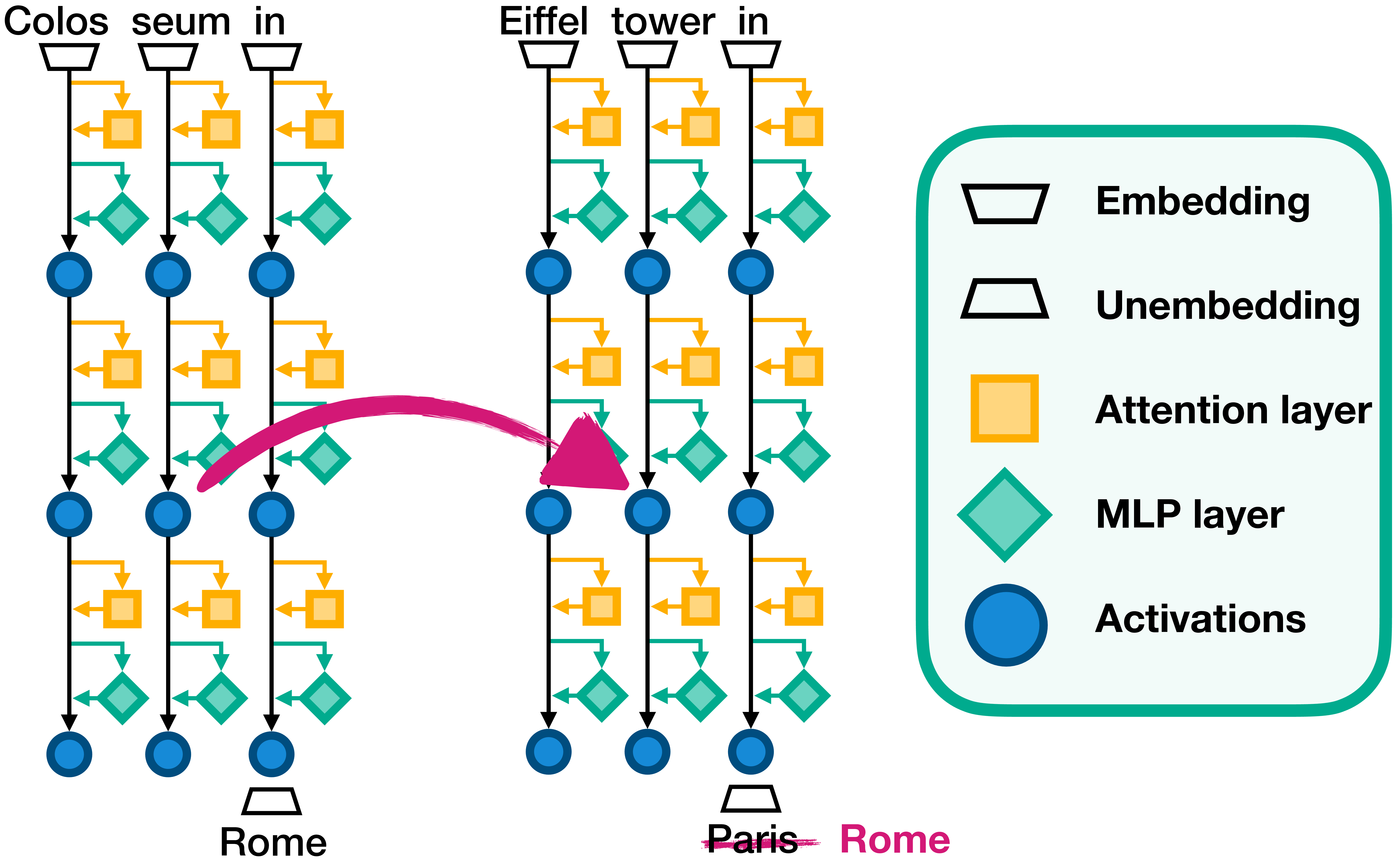
The image below depicts a whole-activation patch: an activation from a run concerning one landmark is inserted into a run concerning another, and the pictured answer changes. It illustrates the causal logic of replacement, but also its interpretive limit: the patched activation may contain multiple differences between the two prompts.
State what would count against each claim
A useful hypothesis records its scope and its possible failure modes in advance. For the carry example, the evidence can be organized as follows:
| Claim | Predicted observation on held-out examples | Result that counts against this claim |
|---|---|---|
| The feature tracks carry at the specified site. | Its score separates carry from no-carry cases across varied digits and formats, including close cases around the threshold. | Separation disappears on those cases, or high scores mostly follow a simpler cue such as a particular digit. |
| The model uses that feature for the tested tens-digit behavior. | A sufficiently selective carry-to-no-carry edit shifts the -versus- margin downward; the reverse edit shifts it upward. | Valid, selective edits have no reliable predicted effect, or effects appear just as strongly for suitable control edits. |
| The feature is a complete carry mechanism. | The proposed feature and its specified downstream route account for the relevant behavior throughout the claimed population. | Carry behavior persists through other routes or the proposed account fails on substantial parts of that population. |
These are not equally strong claims. Failing an output-intervention test does not automatically show that carry information is unreadable: the model may encode it without using it at this site. Equally, an output effect does not prove that the feature is the sole or normal route for carry. A large, unnatural edit may recruit a pathway that matters only under intervention. The conclusion should match the experiment actually performed.
For that reason, a practical prediction record should include the candidate unit and location, the concept’s observable definition, the held-out input population, the expected score or output change, and the alternative cue or intervention artifact that a control should rule out. Your familiarity with hooks makes the location and edit technically concrete; the harder scientific work is specifying what the resulting measurement would mean.
Conclusion
To make “this feature represents a concept” falsifiable, replace the label with scoped predictions. First predict where the feature score should be high and low on independently chosen examples, including near misses. If the claim extends to computation, predict the direction of a behavioral change under a specified, controlled intervention. Keep the conclusions separate: selective activation supports a readout claim; a targeted behavioral effect supports a narrower causal claim on the tested inputs; neither alone establishes a complete mechanism.
The next lesson develops matched examples more carefully, especially cases that vary a suspected shortcut cue while preserving the evidence the task legitimately requires.