Hello. In the previous lesson, you kept a trained probe fixed and tested it where a nuisance cue became misleading. That test can expose a fragile readout. But even with a well-designed test set, a comparison between layers can mislead if the probes differ in what they are capable of learning or how much data they receive.
This lesson is about diagnosing that problem. You will examine how readout capacity, activation dimension, and sample size affect a layerwise result, then build a comparison protocol that makes its remaining limitations explicit. Allow about 40 minutes, including the readings.
A probe score belongs to a configuration, not just a layer
Suppose a linear probe trained on layer 4 reaches 90% accuracy, while a probe trained on layer 12 reaches 93%. It is tempting to say that layer 12 represents the target more clearly. First ask what else changed. Was the second probe an MLP? Were its activation vectors larger? Did it receive more training examples?
A probe result depends jointly on the representation, readout family, training data, and evaluation procedure. If several of those change at once, the accuracy difference cannot be assigned to the layer alone. This remains true when both probes are evaluated on exactly the same held-out examples: a matched test set removes one source of unfairness, not all of them.
For a binary linear readout of a -dimensional activation, the weight vector and bias contain trainable parameters. A 256-dimensional input gives 257 parameters; a 2,048-dimensional input gives 2,049. Both readouts are called “linear,” but they have different numbers of adjustable weights and access to different input spaces. That does not mean the larger one will necessarily perform better. It means that “same probe architecture” is not, by itself, a complete account of capacity.
Capacity also depends on the function family. A one-hidden-layer MLP can learn nonlinear decision boundaries that a linear probe cannot. Increasing hidden width, reducing regularization, or training longer can change what the readout extracts. Thus, a higher MLP score may show that information can be recovered by a more capable computation, rather than that it is more directly linearly readable.
The following paper makes this distinction concrete. Read its probe definitions and complexity controls before its layer comparison.
[PDF] Designing and Interpreting Probes with Control Tasks - ACL Anthology
Read Hewitt and Liang’s paper to see how probe design affects both task accuracy and the interpretation of a layerwise ranking.
In Section 3.1, “Probe families,” find the paragraph beginning “We experiment with three types of probes per task.” Read the probe definitions for part-of-speech tagging, distinguishing the linear readout from the MLPs. Then, in Section 3.2, “Complexity control,” read the rank, width, and dropout controls, followed by the “Number of training examples” paragraph through its explanation of sample efficiency. In Section 4, “Selectivity Differences Confound Layer Comparisons” (around printed p. 2740), locate the paragraph beginning “In particular, word identities are strong features.” Read the proposed confound. In Section 4.2, “Results & Discussion,” read from the comparison of the two ELMo layers through the accuracy and selectivity figures. Focus on why the small accuracy advantage and the selectivity advantage point in different directions.
The paper’s example is instructive because the question is not simply whether a probe can tag parts of speech. A readout might also exploit accessible word identity to predict a word’s usual tag. The authors’ control task tests whether the probe can learn assigned labels tied to word types; selectivity compares performance on the linguistic task with performance on that control. Their linear probe scores 97.2% part-of-speech accuracy on one layer and 96.6% on the other, yet the latter has higher reported selectivity: 31.4 rather than 26.0. Accuracy alone and accuracy considered alongside this control support different interpretations.
Selectivity is a diagnostic, not a universal correction factor. A control task probes the particular shortcut or memorization route it was designed to expose. A more selective layer has not thereby been proved to contain a uniquely identifiable “part-of-speech feature,” nor has a less selective layer been proved to lack one.
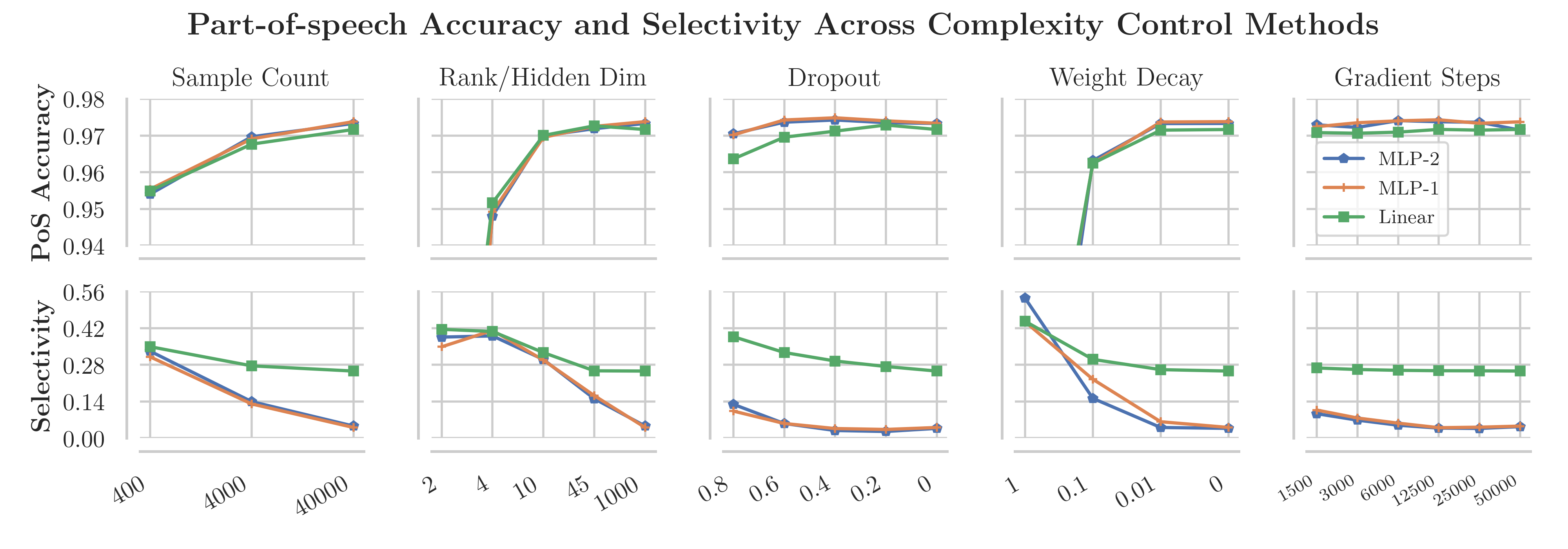
Notice the separate Sample Count panels in the figure. More training examples bring strong task accuracy, while selectivity for the MLP probes falls markedly across the displayed range. The lesson is not that a small training set is automatically preferable. It is that changing sample count can change which strategy the probe learns, even when the task score looks healthy. A layer comparison that gives its probes different amounts of data may therefore compare different learning opportunities.
Three confounds to diagnose
Consider this hypothetical report. Both rows use the same held-out test set.
| Site | Activation width | Probe | Training examples | Test accuracy |
|---|---|---|---|---|
| Earlier layer | 256 | Linear | 4,000 | 90% |
| Later layer | 2,048 | MLP, width 64 | 16,000 | 93% |
The 93% score is a genuine score for that configuration. It does not isolate a layer advantage.
Readout capacity. The MLP can implement functions unavailable to the linear probe. For binary output, a 2,048-input, width-64 MLP with biases has 131,201 trainable parameters, versus 257 for the earlier layer’s linear probe. Parameter count is an imperfect measure of effective capacity, but this difference is too large to ignore. A useful diagnosis is to compare both layers with the same readout family, and then report how their scores change as permitted capacity varies.
Activation dimension. Even two linear probes may have unequal input widths. A wider activation offers more coordinates in which a signal—or an incidental correlate—could be found. It may also require more data to estimate a reliable readout. Do not “fix” this silently by projecting the wider layer to 256 dimensions and reporting only that result: a projection might discard useful information. Instead, report native-width results and, if dimensionality is central to the claim, a clearly labeled sensitivity analysis using the same fixed projection procedure and target dimensions across layers. A learned projection is itself a readout component and must be counted as such.
Training sample size. The later-layer probe has four times as many examples. Its advantage could reflect easier estimation rather than a better representation. Train comparisons on the same source examples, with identical label and nuisance-group composition, and plot performance at several shared training sizes. This reveals whether an apparent ranking holds across the available data range or depends on one allocation.
These controls address different questions. Equalizing example counts does not equalize activation widths; using linear probes does not equalize the data needed to estimate their weights. Nor is a fixed ratio of examples to dimensions a universal fairness rule: correlated coordinates, regularization, and the strength of the signal all matter.
Adequate data for the comparison
Training-set size and test-set size play different roles. Too little training data may leave one probe poorly estimated, especially if its readout has many adjustable parameters. Too little test data may make a small difference between two trained probes impossible to distinguish reliably. A large shared test set cannot rescue undertrained probes, and a large training set cannot make a tiny test set precise.
On the data requirements of probing - ACL Anthology
Read the paper’s two comparison examples to separate data needed to fit a probe from data needed to resolve a difference between probes.
In Section 4.5, “Comparing between encoders,” find the sentence beginning “A test set of size.” Read the test-size comparison and its accompanying Figure 5: the smaller test set does not adequately resolve the reported encoder comparison. Then turn to Section 4.6, “Comparing between classifiers” (around printed p. 4138). Starting where the authors compare a logistic regressor with a one-hidden-layer MLP, read through the parameter-count and data discussion. Focus on why a more flexible classifier and a very small difference in observed scores complicate a claimed ranking. Treat the paper’s numerical requirements as estimates for its particular comparisons, not universal minimum sample sizes.
If two layer probes make predictions on the same test examples, examine the difference as a paired result. Record the accuracy gap, the number of test examples and independent source items, and uncertainty in the gap—not just two rounded percentages. Repeat training with several seeds or shared training subsamples to see whether the ranking is stable. If a small observed advantage varies substantially with those choices, the defensible conclusion is that the comparison is unresolved under the present protocol. Statistical precision and experimental fairness are separate issues: a precisely measured difference between an MLP trained on more data and a smaller linear probe is still confounded.
A defensible layerwise report
A practical comparison can begin with a question narrow enough to test: At which layer is the target easiest to decode with a specified readout under a specified data budget? The report should then make that specification visible.
Use the same frozen model inputs, target definition, source-level train/validation/test split, and held-out evaluation examples for every layer. If the nuisance cue from the previous lesson matters, retain its groups in the report; a layer’s average score can hide failure on conflicting-cue cases. Fit normalization using only the relevant probe-training split, apply the resulting transform unchanged to validation and test, and select regularization on validation data under a comparable search budget. Never choose the winning layer or projection after inspecting the final test results.
For interpretation, report a small capacity-and-data profile rather than only the maximum accuracy: for example, linear probes at shared training sizes, with native activation dimensions and parameter counts stated; optionally add a separately labeled MLP profile. Include the control-task result when memorization of an irrelevant correlate is a plausible explanation. If changing width, regularization, sample size, or readout family reverses the layer ranking, that reversal is a substantive finding: the original ranking depended on the probing setup.
Even a stable, carefully controlled ranking supports a bounded claim about decodability under the tested readouts and data distribution. It does not show that the model’s original output computation uses the decoded information. That distinction will become especially important in the next lesson, which constructs a case where a concept is linearly decodable but unused by the model’s prediction.
Takeaways
A layerwise probe comparison is unfair when an apparent representation difference is entangled with readout capacity, activation dimension, or the number of examples available to fit and evaluate the readout. Diagnose those factors explicitly; compare on shared data; show sensitivity to capacity and training size; and keep uncertainty separate from fairness. A probe can establish that a readout succeeds under specified conditions. Establishing what the model does with that information requires a different test.