Welcome to the probing module. You have already encountered the idea that a model’s internals might contain recognizable concepts; here we begin testing such claims. This module starts with linear probes, then asks whether their apparent success survives stronger controls and changes in context.
In this lesson, you will fit a probe to cached activations, choose its settings on a validation set, and evaluate it once on a held-out test set. The key distinction is between finding information that a new readout can extract and showing that the original model uses that information. Plan on about 45 minutes, including the short resources and running the code.
What a linear probe measures
Suppose each example has a cached activation vector from one fixed location in a frozen model, together with a binary concept label . A linear probe learns a weight vector and bias:
Applying a sigmoid to gives the probe’s predicted probability of the positive label. If it predicts held-out labels well, the label is linearly readable from those activations under the tested data distribution. That is a narrower conclusion than “the model uses this concept to make its prediction.”
Explainability methods: Linear Probes - The Carpentries Incubator
Read “Explainability methods: Linear Probes” from The Carpentries Incubator for the purpose and limits of a simple readout.
In “What part of my model causes this prediction?”, read “Method and Examples” from representations and probes. Then, in “Limitations and Extensions,” read the usage caveat. Focus on the difference between information available to a probe and information used by the original model.
For an interpretability study, define the measurement before fitting: which model, which layer or component, which token position, and what the label means. For example, you might cache the residual-stream vector at the final prompt token and ask whether a property of the prompt is readable there. If the answer or label appears later in the input whose activations you cache, the probe may solve a different, trivial task.
Splits are part of the claim
A probe can fit training examples without learning a relationship that generalizes. Training, validation, and test sets therefore have different jobs: fit weights on training data, choose settings such as regularization and stopping point using validation data, and reserve test data for one final estimate after those choices are fixed.
Why do we split data into train test and validation sets?
Watch “Why do we split data into train test and validation sets?” by Mısra Turp for a quick account of the three roles and why the splitting method matters.
Watch the three roles, then split strategy. Treat the percentages given as an example, not a required ratio. In this lesson, “validation” always means data used to choose a probe; “test” means data kept out of that choice.
For cached activations, which examples are independent matters as much as the proportions. Imagine four paraphrases of the same source sentence. If two enter training and two enter testing, a probe might recognize source-specific details rather than the proposed concept. Assign all four a group ID and keep the entire group in one partition. Depending on the dataset, a group might be a source document, an original prompt and its variants, or another shared origin that could make examples dependent.
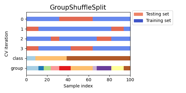
A split alone does not prevent all leakage. If you standardize activation dimensions using a mean and standard deviation computed from all examples, the held-out activations have influenced preprocessing. Fit those statistics on training activations only; apply the same transformation unchanged to validation and test activations.
3.1. Cross-validation: evaluating estimator performance
Read two targeted passages in scikit-learn’s “Cross-validation: evaluating estimator performance” to connect group-aware splitting with train-only preprocessing.
Within “3.1.1. Computing cross-validated metrics,” open “Data transformation with held-out data.” Read from train-only transformations through its standardization example. Then go to “3.1.2.4. Cross-validation iterators for grouped data” and read the grouped-data premise. Focus on what information each split is permitted to contribute.
Fit a probe in PyTorch
The following runnable example creates a stand-in activation cache: 120 independent groups, each with four related samples and a 16-dimensional vector. A binary signal is present alongside group-specific variation and noise. In a real study, replace only the cache-generation section with your frozen model’s saved activations, labels, and group IDs; keep the splitting and probe-fitting logic.
The outer group split reserves the test groups. A second group split divides the remainder into training and validation groups. The code then fits normalization statistics on training activations, trains several regularized linear probes, selects by validation loss, and finally reports test accuracy alongside a training-majority-class baseline.
import copy

import numpy as np
import torch
import torch.nn as nn
import torch.nn.functional as F
from sklearn.model_selection import GroupShuffleSplit

torch.manual_seed(17)

# Stand-in for a frozen model's cached activations.
n_groups, examples_per_group, d = 120, 4, 16
groups = torch.arange(n_groups).repeat_interleave(examples_per_group)
y = (groups % 2).long()

group_offset = torch.randn(n_groups, d)
concept_direction = torch.zeros(d)
concept_direction[0] = 1.0

X = (
    1.3 * (2 * y.float() - 1)[:, None] * concept_direction
    + 0.7 * group_offset[groups]
    + 0.65 * torch.randn(len(groups), d)
).detach()

# Split by group, not by row. The outer test set stays untouched
# during preprocessing, training, and model selection.
rows = np.arange(len(groups))
group_ids = groups.numpy()

outer = GroupShuffleSplit(n_splits=1, test_size=0.20, random_state=31)
trainval_idx, test_idx = next(
    outer.split(rows, y.numpy(), group_ids)
)

inner = GroupShuffleSplit(n_splits=1, test_size=0.25, random_state=32)
train_rel, val_rel = next(
    inner.split(
        trainval_idx,
        y[trainval_idx].numpy(),
        group_ids[trainval_idx],
    )
)
train_idx = trainval_idx[train_rel]
val_idx = trainval_idx[val_rel]

split_groups = [
    set(groups[idx].tolist())
    for idx in (train_idx, val_idx, test_idx)
]
assert split_groups[0].isdisjoint(split_groups[1])
assert split_groups[0].isdisjoint(split_groups[2])
assert split_groups[1].isdisjoint(split_groups[2])

# Fit the transformation on training activations only.
mean = X[train_idx].mean(dim=0)
scale = X[train_idx].std(dim=0, unbiased=False).clamp_min(1e-6)
X_scaled = (X - mean) / scale

def fit_probe(weight_decay, epochs=200):
    # Same initialization across settings makes this comparison less noisy.
    torch.manual_seed(23)
    probe = nn.Linear(d, 1)
    optimizer = torch.optim.Adam(probe.parameters(), lr=0.03)

    best_val_loss = float("inf")
    best_state = None
    best_epoch = None

    for epoch in range(epochs):
        probe.train()
        logits = probe(X_scaled[train_idx]).squeeze(-1)
        train_loss = F.binary_cross_entropy_with_logits(
            logits, y[train_idx].float()
        )
        loss = train_loss + weight_decay * probe.weight.square().sum()

        optimizer.zero_grad()
        loss.backward()
        optimizer.step()

        probe.eval()
        with torch.no_grad():
            val_logits = probe(X_scaled[val_idx]).squeeze(-1)
            val_loss = F.binary_cross_entropy_with_logits(
                val_logits, y[val_idx].float()
            ).item()

        if val_loss < best_val_loss:
            best_val_loss = val_loss
            best_state = copy.deepcopy(probe.state_dict())
            best_epoch = epoch + 1

    probe.load_state_dict(best_state)
    probe.eval()
    return best_val_loss, best_epoch, probe

candidates = []
for strength in (0.0, 0.001, 0.01, 0.1):
    val_loss, epoch, probe = fit_probe(strength)
    candidates.append((val_loss, strength, epoch, probe))

best_val_loss, strength, epoch, probe = min(
    candidates, key=lambda result: result[0]
)

# Only now score the held-out test groups.
with torch.no_grad():
    test_logits = probe(X_scaled[test_idx]).squeeze(-1)
    test_predictions = (test_logits >= 0).long()
    test_accuracy = (
        (test_predictions == y[test_idx]).float().mean().item()
    )

majority_label = torch.bincount(y[train_idx], minlength=2).argmax()
majority_accuracy = (
    (y[test_idx] == majority_label).float().mean().item()
)

print("groups per split:", [len(part) for part in split_groups])
print("chosen regularization:", strength)
print("chosen epoch:", epoch)
print("validation loss:", round(best_val_loss, 4))
print("test accuracy:", round(test_accuracy, 4))
print("test majority baseline:", round(majority_accuracy, 4))
A single nn.Linear layer is the probe: there are no hidden layers that could construct a nonlinear representation. BCEWithLogitsLoss supplies the binary classification objective without requiring a separate sigmoid during training. A nonzero regularization strength penalizes large readout weights; both that strength and the saved training epoch are chosen using validation data, not test accuracy.
For a real activation cache, make X a tensor with one row per example, y its aligned binary-label tensor, and groups its aligned dependency IDs. Cache at the same defined site for every example, with the original model in evaluation mode and without training it through the probe. Store enough metadata to verify that each row’s activation, label, source group, and token position still match.
Interpreting the result without overclaiming
The synthetic cache was built with a learnable signal, so it is useful for checking whether the pipeline can recover one. It does not validate a claim about an actual transformer. On real activations, record the chosen site and label definition, group rule, split seed, preprocessing, selection criterion, test score, and baseline. A score above the baseline on held-out groups supports the claim that this linear readout can predict those labels on those groups.
Two boundaries remain. First, a good test score does not establish that the original model reads out the same direction—or uses the labeled concept at all. Second, group-disjoint evaluation addresses the dependencies represented by your group IDs, not every possible shortcut in the dataset. Those are reasons to make the claim precise, not reasons to discard the measurement.
A leakage-resistant probe begins with a fixed activation-and-label definition, keeps dependent examples together, learns preprocessing and weights from training data, selects using validation data, and consults test data only after selection. Its result is evidence about readability, not yet about causal use. The next lesson introduces a control-label baseline to test whether apparent probe success reflects meaningful structure rather than the readout’s ability to fit an uninformative labeling scheme.