Gradient Descent: Derivation and Convergence for Convex Functions

The Intuition: Approximating and Stepping

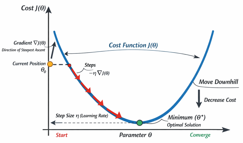
The core idea of gradient descent is simple: start somewhere, look around to see which way is "downhill," and take a step in that direction. We repeat this process until we can't go any lower. To make this precise, we need a mathematical way to determine the "downhill" direction.

This is where the Taylor series, a powerful tool for approximating functions, comes into play. A first-order Taylor approximation allows us to approximate a complex function near a point with a simple linear function—its tangent line (or hyperplane in higher dimensions).

To refresh your intuition on using simpler functions for approximation, this video by Dr. Trefor Bazett provides a great conceptual overview.

As the video shows, the linear approximation $f(a)+f^{\prime }(a)(x-a)$ is the best linear fit to the function $f(x)$ near the point $a$. We will use this exact idea to decide which direction to move from our current position.

Deriving the Gradient Descent Update Rule

Let's formalize the "downhill" search. Suppose we are at a point ${\mathbf{x}}_t$ and we want to find a new point ${\mathbf{x}}_{t+1}={\mathbf{x}}_t+\mathbf{p}$ such that $f({\mathbf{x}}_{t+1})<f({\mathbf{x}}_t)$. We'll define our step $\mathbf{p}$ as $\eta \mathbf{d}$, where $\eta >0$ is a small scalar called the step size or learning rate, and $\mathbf{d}$ is a unit vector representing the direction of movement.

Using a first-order Taylor expansion around ${\mathbf{x}}_t$, we can approximate the function value at the new point:

The change in the function value is therefore:

Our goal is to make this change as negative as possible to ensure the greatest decrease in $f$. Since $\eta$ is a positive constant, we need to choose the direction $\mathbf{d}$ to minimize the quantity $\nabla f({\mathbf{x}}_t{)}^T\mathbf{d}$.

This video provides an excellent and intuitive walkthrough of this exact derivation for a single-variable function.

As the video concludes, to make the product $\nabla f({\mathbf{x}}_t{)}^T\mathbf{d}$ most negative, we should choose $\mathbf{d}$ to be in the direction opposite to the gradient $\nabla f({\mathbf{x}}_t)$.

More formally, from the definition of the dot product (and the Cauchy-Schwarz inequality), we know:

where $\theta$ is the angle between the gradient and the direction vector. Since $\mathbf{d}$ is a unit vector ($||\mathbf{d}||=1$), this expression is minimized when $\cos (\theta )=-1$. This occurs when $\mathbf{d}$ points in the exact opposite direction of $\nabla f({\mathbf{x}}_t)$.

Thus, the direction of steepest descent is $\mathbf{d}=-\frac{\nabla f({\mathbf{x}}_t)}{||\nabla f({\mathbf{x}}_t)||}$.

Plugging this back into our step, $\mathbf{p}=\eta \mathbf{d}$, we get the update rule:

In practice, the normalization term $||\nabla f({\mathbf{x}}_t)||$ is often absorbed into the learning rate $\eta$, giving us the canonical gradient descent update rule:

Convergence Guarantees of Gradient Descent

We've derived a plausible algorithm, but does it actually work? Under what conditions will it converge to the minimum ${\theta }^{\ast }$? This is where we connect back to the properties of the function we are optimizing.

The proofs of convergence typically rely on an assumption called L-smoothness.

Definition (L-smoothness): A differentiable function $f$ is L-smooth if its gradient is Lipschitz continuous with constant $L\ge 0$. This means for any two points $\mathbf{x}$ and $\mathbf{y}$:

Intuitively, L-smoothness means the gradient cannot change arbitrarily fast. A key consequence is that an L-smooth function is upper-bounded by a quadratic function. This "quadratic upper bound" is essential for the analysis.

To understand the convergence proof, we'll follow the clear and rigorous derivation in the MIT lecture notes by Prof. Gabriele Farina.

Let's break down the key results from that reading:

1. Descent Lemma (for L-smooth functions): If $f$ is L-smooth and we choose a step size $0<\eta \le 1/L$, then each step of gradient descent guarantees progress:

   $$f({\mathbf{x}}_{t+1})\le f({\mathbf{x}}_t)-\frac{\eta }{2}||\nabla f({\mathbf{x}}_t)|{|}^2$$

   This tells us the function value will decrease at every step unless the gradient is zero (i.e., we are at a stationary point). For a non-convex function, this could be a local minimum or a saddle point.

2. Convergence for Convex Functions (Theorem 2.6): When we add the assumption that $f$ is also convex, we can prove a much stronger result. As derived in the notes, the sub-optimality of the function value (the difference between the current value and the true minimum $f({\mathbf{x}}^{\ast })$) is bounded:

   $$f({\mathbf{x}}_t)-f({\mathbf{x}}^{\ast })\le \frac{||{\mathbf{x}}_0-{\mathbf{x}}^{\ast }|{|}^2}{2t\eta }$$

   This is a profound result. It guarantees that gradient descent will converge to the global minimum. The rate of this convergence is $O(1/t)$, which is known as a sublinear rate. This means that to achieve a desired accuracy $ϵ$, we need approximately $O(1/ϵ)$ iterations.

A Note on Faster Convergence

While $O(1/t)$ convergence is good, we can do even better under a stronger condition called m-strong convexity. An m-strongly convex function is one whose curvature is bounded below by some $m>0$ (formally, ${\nabla }^{2}f(\mathbf{x})⪰mI$). For such functions, gradient descent enjoys a linear convergence rate.

As shown in the reading, for an L-smooth and m-strongly convex function, the convergence rate is:

This is an exponential decay, often written as $O({\rho }^t)$ where $\rho <1$. This means we only need $O(\log (1/ϵ))$ iterations to reach an accuracy of $ϵ$, which is significantly faster than the sublinear rate for general convex functions.

Conclusion

In this lesson, we demystified the gradient descent algorithm. You learned not just what it does, but why it works. The key takeaways are:

• The gradient descent update rule, ${\mathbf{x}}_{t+1}={\mathbf{x}}_t-\eta \nabla f({\mathbf{x}}_t)$, is derived by minimizing a first-order Taylor approximation of the function at the current point.
• The negative gradient, $-\nabla f(\mathbf{x})$, is the direction of steepest descent.
• Convergence is not automatic. It depends on the properties of the function being optimized.
• For an L-smooth and convex function, gradient descent is guaranteed to converge to the global minimum with a sublinear rate of $O(1/t)$.
• If the function is also m-strongly convex, the convergence rate improves exponentially to a linear rate, $O({\rho }^t)$.

So far, we have assumed that we can compute the full gradient $\nabla f(\mathbf{x})$ at each step. This involves evaluating the gradient over all data points in your training set. For massive datasets, this can be computationally prohibitive. In our next lesson, we will address this challenge by exploring Stochastic Gradient Descent (SGD), a powerful and widely used variant that approximates the gradient using only a small subset of the data.