Breadth-First Search (BFS) on Graphs

The Intuition: Exploring in Ripples

Imagine dropping a stone into a still pond. The ripples spread out from the center in perfect, expanding circles. Breadth-First Search explores a graph in the exact same way. It starts at a source node and "visits" it. Then it visits all of the source's immediate neighbors. Then it visits all of their unvisited neighbors, and so on. It explores "broadly" across the graph, one level of connections at a time, before going any deeper.

This level-by-level approach is the defining characteristic of BFS. Let's look at a visual representation of this process.

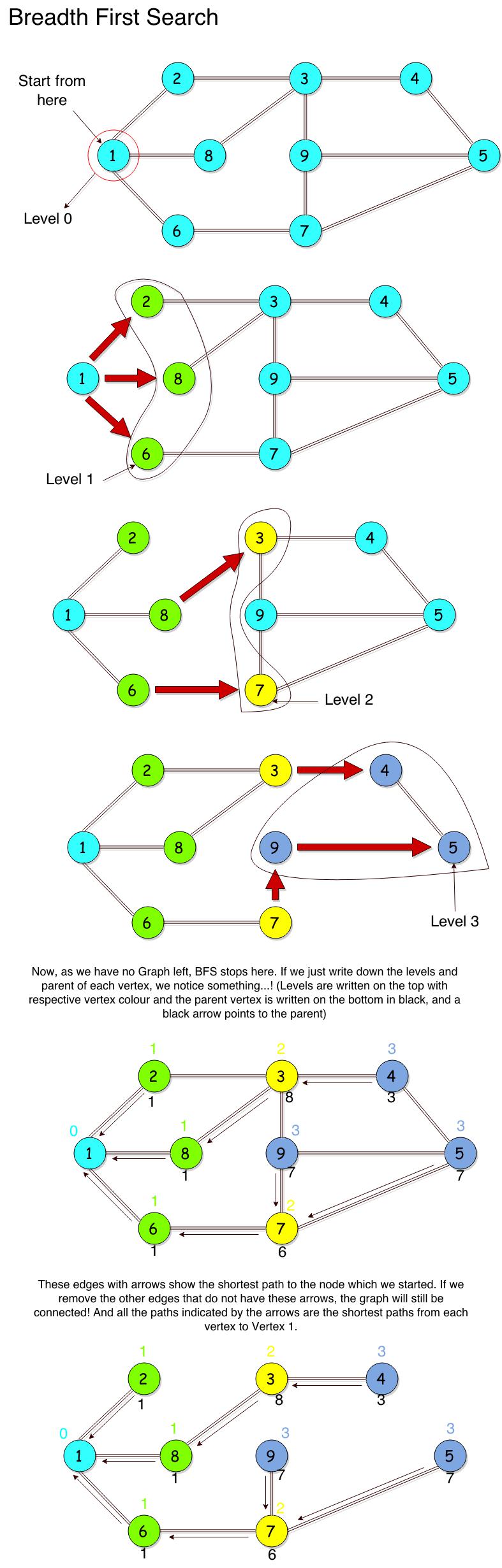
This method has a very important consequence: by exploring level by level, BFS naturally finds the shortest path from the source node to all other nodes, if we measure the path length simply by the number of edges.

The following video provides an excellent analogy to help this idea click and solidifies the concept of exploring level-by-level.

As the video explains, the moment BFS reaches a node, it has found the shortest path to that node from the source. This property makes BFS the go-to algorithm for shortest path problems in unweighted graphs, a topic we will explore in a future lesson.

The Algorithm: Queues and Visited Sets

Now that we have the intuition, let's make it concrete. How do we program a computer to explore a graph level by level? The answer lies in two simple data structures:

1. A Queue: This is a "First-In, First-Out" (FIFO) data structure. Think of it as a line at a checkout counter. The first person to get in line is the first one served. In BFS, the queue keeps track of the nodes we need to visit next. By always processing nodes in the order they were discovered, we ensure the level-by-level traversal.
2. A Visited Set: This is a set (or a boolean array) that keeps track of the nodes we have already visited or have already added to our queue. This is crucial to avoid processing the same node multiple times and to prevent getting stuck in infinite loops in graphs with cycles.

The algorithm proceeds as follows:

1. Initialize: Choose a starting node. Add it to the queue and mark it as visited.
2. Loop: While the queue is not empty:
   a. Dequeue: Remove the node from the front of the queue. Let's call this the current_node.
   b. Process: Do something with current_node (e.g., print its value).
   c. Explore Neighbors: For each neighbor of current_node:
   i. If the neighbor has not been visited:
   ii. Mark it as visited and add it to the back of the queue.
3. Terminate: Once the queue is empty, all reachable nodes have been visited.

Let's see this process in action. The following video provides a clear, animated walkthrough of the BFS algorithm on a sample graph.

To connect the code, the graph, and the data structures, take a look at the image below. It provides a snapshot of the algorithm at a single point in time.

Here, node 5 has just been dequeued. The queue contains nodes 4, 3, and 6, which are on the "frontier" to be explored next. The visited set shows all nodes that have been discovered so far. This visual perfectly captures the state of a BFS traversal.

Complexity and Contrast

As a data scientist, understanding the performance of an algorithm is key. BFS is highly efficient. For a graph with $V$ vertices and $E$ edges, the complexity is:

• Time Complexity: $O(V+E)$. This is because, in the worst case, we visit every vertex once and cross every edge once. We don't re-process anything thanks to the visited set.
• Space Complexity: $O(V)$. In the worst case, the queue could hold all vertices of a particular level. For a dense graph, this could be on the order of $V$ vertices. The visited set also requires $O(V)$ space.

The following resource provides a good explanation for why the time complexity is additive ($V+E$) rather than multiplicative ($V\times E$).

It's useful to know that BFS is not the only way to traverse a graph. Its counterpart is Depth-First Search (DFS). While BFS uses a queue to explore widely, DFS uses a stack (Last-In, First-Out) to explore deeply, going as far as it can down one path before backtracking. We will cover DFS in detail in our next lesson.

Conclusion

In this lesson, we demystified the Breadth-First Search algorithm. We moved from a high-level, intuitive understanding of its "ripple-like" exploration to the concrete mechanics of its implementation with a queue and a visited set.

Here are the key takeaways:

• BFS explores a graph level by level, starting from a source node.
• It relies on a queue (FIFO) to maintain the order of nodes to visit, ensuring a "wide" traversal.
• A visited set is essential to avoid redundant processing and infinite loops.
• A key application of BFS is finding the shortest path in terms of edge count in unweighted graphs.
• The algorithm is efficient, with a time and space complexity of $O(V+E)$ and $O(V)$ respectively.

In our next lesson, we'll dive into Depth-First Search (DFS). You'll see how swapping the queue for a stack leads to a completely different traversal strategy and enables a different set of applications, such as cycle detection and topological sorting.