Welcome to the second lesson in our journey into Graph Neural Networks. In our previous discussion, we established the abstract language of graphs, defining them as a set of vertices and edges . Now, we will bridge the gap between this abstract concept and a concrete implementation. Before we can run any algorithm or build a neural network, we must decide how to store a graph's structure in a computer's memory.
This lesson focuses on answering that fundamental question. You will learn about the two most common and essential methods for representing graphs: the adjacency matrix and the adjacency list. Understanding the trade-offs between these representations is not just an academic exercise; it's a critical decision that impacts memory usage and algorithmic efficiency, especially for the large-scale graphs you'll encounter in real-world applications.
The Adjacency Matrix: A Direct Translation
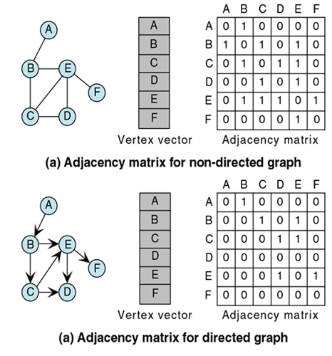
The most straightforward way to represent a graph is with an adjacency matrix. For a graph with nodes, we create a square matrix, let's call it . The rule is simple:
For weighted graphs, instead of storing a 1, we would store the edge's weight. This representation provides a direct, tabular view of the graph's connectivity.
The image below illustrates how both an undirected and a directed graph are translated into their corresponding adjacency matrices.
To see a step-by-step construction of adjacency matrices, the following video provides clear examples for different graph types.
Graph Neural Networks (GNN) | Nodes, Edges, Adjacency Matrix, Message Passing, Aggregation explained
Watch these segments from the Vizuara channel's video on GNNs. They meticulously walk through the process of creating an adjacency matrix for directed, undirected, and weighted graphs.
Pay close attention to the logic for placing 0s and 1s (or weights): Building the matrix for a directed graph. Note how the direction of the edge determines which cell gets a '1'. Building the matrix for an undirected graph. Observe how this results in a symmetric matrix. Building the matrix for a weighted graph. This shows how the '1' is replaced by the edge's actual weight.
While intuitive, the adjacency matrix has significant performance implications. The following reading provides a sharp analysis of its strengths and weaknesses.
Graph Representations: Adjacency Matrix, List & More
This article from TensorTonic provides an excellent breakdown of the adjacency matrix, including its properties and a complexity analysis that is crucial for any data scientist.
Please read the section titled "Adjacency Matrix". Focus on the "Complexity Analysis" table and the "Matrix Powers" property. The idea that A^k counts paths of length k is a powerful concept that is fundamental to how information propagates in GNNs.
As you've just read, the primary drawback of the adjacency matrix is its space complexity of . For a social network with a million users, this is infeasible. This is because most real-world graphs are sparse—the number of actual connections is far less than the number of possible connections. Storing a massive matrix of mostly zeros is highly inefficient.
The Adjacency List: An Efficient Alternative for Sparse Graphs
To solve the space problem, we can use an adjacency list. Instead of a matrix representing all possible connections, we only store the connections that actually exist. For each node, we maintain a list of its neighbors.
This can be implemented in various ways, but a common approach in Python is to use a dictionary (or hash map) where keys are the nodes and values are lists of their adjacent nodes.

The adjacency list representation is far more memory-efficient for the sparse graphs common in machine learning. Its space complexity is , where is the number of edges. This is a dramatic improvement over the adjacency matrix's .
This next video will help you solidify your understanding of the adjacency list and contrast it with the matrix.
Graphs: Edge List, Adjacency Matrix, Adjacency List, DFS, BFS - DSA Course in Python Lecture 11
This clip from Greg Hogg's DSA course explains the adjacency list concept and why it's often preferred.
Watch from this section where he introduces the adjacency list as a hash map, which is a very practical and common implementation you'll use.
Now, let's return to the TensorTonic article to analyze the performance characteristics of the adjacency list.
Graph Representations: Adjacency Matrix, List & More
This section details the adjacency list, its implementation choices, and complexity.
Read the section titled "Adjacency List". Again, focus on the "Complexity Analysis" table. Notice the trade-off: finding a specific edge is now potentially slower than with a matrix, but iterating over all of a node's neighbors is much faster.
The Core Trade-off: Making the Right Choice
As a data scientist, choosing the right data structure is a classic engineering trade-off. There is no single "best" representation; the choice depends on the graph's properties and the operations you need to perform.
| Representation | Space | Check Edge (i, j) | Get Neighbors of i | Best For |
|---|---|---|---|---|
| Adjacency Matrix | Dense graphs, linear algebra | |||
| Adjacency List | Sparse graphs, graph traversal |
Note: is the degree of node , or the number of its neighbors.
For most GNN applications on large, sparse graphs, the adjacency list (or a similar sparse format) is the clear winner for storing the graph structure. However, the concept of the adjacency matrix is still vital. The core operation in many GNNs, message passing, can be mathematically formulated as a multiplication with the adjacency matrix.
The Distill article on GNNs provides a great perspective on this specific challenge in machine learning.
A Gentle Introduction to Graph Neural Networks
This article explains why representing graph connectivity is a unique challenge for neural networks.
First, read the section "The challenges of using graphs..." to understand why adjacency matrices are often inefficient and how adjacency lists offer a memory-friendly solution. Then, read the first two paragraphs of the section "Graph convolutions as matrix multiplications...". This part is key: it shows that even if we use an adjacency list for storage, the underlying mathematical operation of a graph convolution is equivalent to a matrix multiplication with the adjacency matrix. This connects today's topic directly to the "neural network" part of GNNs.
From Theory to Practice: Python Implementation
Given your goal of implementing GNNs, let's see how you would build these representations in code. A common starting point is an edge list, which is simply a list of tuples, where each tuple (u, v) represents an edge.
The following video segments demonstrate how to convert an edge list into both an adjacency matrix and an adjacency list in Python. The use of defaultdict for the adjacency list is a standard and efficient pattern.
Graphs: Edge List, Adjacency Matrix, Adjacency List, DFS, BFS - DSA Course in Python Lecture 11
In this final viewing, Greg Hogg provides clear, concise Python code for building both representations from an array of edges.
Watch the implementation of an adjacency matrix. Pay attention to how a 2D list is initialized and then populated by iterating through the edges. Watch the implementation of an adjacency list. The use of collections.defaultdict(list) is a powerful Python idiom that simplifies the code significantly.
Conclusion
You have now learned how to translate abstract graphs into concrete data structures. This is the essential prerequisite for performing any computation on graph data.
Here are your key takeaways from this lesson:
- Adjacency Matrix: A matrix that is simple to understand and allows for edge lookups. Its space complexity makes it unsuitable for large, sparse graphs.
- Adjacency List: A more memory-efficient representation with space complexity, ideal for sparse graphs. It excels at iterating through a node's neighbors.
- The Trade-off: The choice between them is a classic space-vs-time decision. For most real-world graphs, an adjacency list or a related sparse format is preferred for storage.
- Relevance to GNNs: While we may store graphs as lists, the mathematical foundation of graph convolutions is deeply connected to the properties of the adjacency matrix.
In our next lesson, we will continue building our graph theory toolkit by defining fundamental node properties like degree and neighbors, and formalizing the concept of weighted edges. These concepts are directly derived from the representations you learned today and are crucial for understanding more advanced graph algorithms.