The Power Method: Iteration and Convergence

Welcome to your first lesson on the numerical computation of eigenvalues. In many real-world applications, finding the eigenvalues of a matrix by analytically solving the characteristic equation is computationally expensive or even impossible, especially for large matrices. This is where numerical methods become essential.

Today, we will explore the Power Method, an elegant and fundamental iterative algorithm. Our goal is to understand the core principle that makes it work and the specific conditions required for it to successfully converge. By the end of this lesson, you will be able to explain how repeated matrix multiplication can reveal a matrix's most dominant characteristic—its largest eigenvalue and the corresponding eigenvector.

The Core Principle: Amplifying the Dominant Eigenvector

The power method is built on a simple yet powerful idea: repeatedly applying a matrix to a vector will gradually amplify the vector's component that aligns with the matrix's "preferred" direction. This preferred direction is precisely the one defined by the eigenvector associated with the eigenvalue of the largest magnitude.

Let's formalize this. Given an $n \times n$ matrix $A$ , we assume it is diagonalizable. This means it has a set of $n$ linearly independent eigenvectors, $v_{1}, v_{2}, \dots, v_{n}$ , corresponding to eigenvalues $λ_{1}, λ_{2}, \dots, λ_{n}$ .

Because the eigenvectors form a basis for $R^{n}$ , any arbitrary non-zero vector $x_{0}$ can be written as a linear combination of these eigenvectors:

x_{0} = c_{1} v_{1} + c_{2} v_{2} + \dots + c_{n} v_{n}

where the coefficients $c_{i}$ are scalars.

What happens when we multiply $x_{0}$ by $A$ ?

A x_{0} = A (c_{1} v_{1} + c_{2} v_{2} + \dots + c_{n} v_{n}) = c_{1} (A v_{1}) + c_{2} (A v_{2}) + \dots + c_{n} (A v_{n})

Since $v_{i}$ is an eigenvector, we know that $A v_{i} = λ_{i} v_{i}$ . Substituting this in, we get:

A x_{0} = c_{1} λ_{1} v_{1} + c_{2} λ_{2} v_{2} + \dots + c_{n} λ_{n} v_{n}

If we multiply by $A$ again, we get $A^{2} x_{0}$ , and after $k$ multiplications, the pattern becomes clear:

A^{k} x_{0} = c_{1} λ_{1}^{k} v_{1} + c_{2} λ_{2}^{k} v_{2} + \dots + c_{n} λ_{n}^{k} v_{n}

This equation is the heart of the Power Method. To understand its implications, let's explore the provided resources.

Eigenvalue Power Method | Lecture 30 | Numerical Methods for Engineers

First, watch this segment from a lecture by Jeffrey Chasnov. It provides a clear verbal walkthrough of the derivation we just covered.

Pay close attention to the derivation from the start up to the point where the general form for A^p \mathbf{x}_0 is established.

9.3. The power method — Linear algebra - Interactive textbooks

Now, read a short section from the TU Delft interactive textbook on linear algebra. This text formalizes the concept and introduces the crucial idea of a "dominant" eigenvalue.

In the section "The basics," please read from the beginning of the derivation to see how the repeated application of matrix A isolates the dominant component.

Dominance and Convergence

As you've just seen, the method's success hinges on one of the eigenvalues being "dominant".

Definition: Dominant Eigenvalue
An eigenvalue $λ_{1}$ is called the dominant eigenvalue if it is strictly greater in absolute value than all other eigenvalues.

∣ λ_{1} ∣ > ∣ λ_{2} ∣ \geq ∣ λ_{3} ∣ \geq \dots \geq ∣ λ_{n} ∣

The corresponding eigenvector $v_{1}$ is called the dominant eigenvector.

Let's rewrite our key equation by factoring out $λ_{1}^{k}$ :

A^{k} x_{0} = λ_{1}^{k} (c_{1} v_{1} + c_{2} (\frac{λ _{2}}{λ _{1}})^{k} v_{2} + \dots + c_{n} (\frac{λ _{n}}{λ _{1}})^{k} v_{n})

Because $λ_{1}$ is dominant, the ratio $∣ λ_{i} / λ_{1} ∣$ is less than 1 for all $i > 1$ . As $k$ becomes large, the terms $(λ_{i} / λ_{1})^{k}$ approach zero.

Assuming $c_{1} \neq = 0$ , the expression in the parentheses converges to $c_{1} v_{1}$ . Therefore, for large $k$ :

A^{k} x_{0} \approx c_{1} λ_{1}^{k} v_{1}

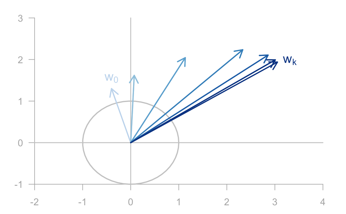
This means that the vector $A^{k} x_{0}$ becomes increasingly aligned with the direction of the dominant eigenvector $v_{1}$ .

The following image provides a great visual for this process. Starting with an initial vector $w_{0}$ , each multiplication by the matrix "pulls" the resulting vector closer to the direction of the dominant eigenvector, which the final vectors, like $w_{k}$ , are approaching.

An illustration of the Power Method. An initial vector $\mathbf{w}_0$ is repeatedly multiplied by a matrix. The resulting vectors are scaled and converge towards the direction of the dominant eigenvector.

To get a more dynamic feel for this "pulling" effect, the next video offers an excellent geometric explanation.

Power Method for Dominant Eigenvalues and Eigenvectors | Linear Algebra

Watch this clip from Wrath of Math for a powerful geometric intuition behind why the method converges.

The segment starts at the explanation of the geometric intuition. The narrator breaks down matrix multiplication into projections onto eigenspaces and scaling, showing visually how the vector is drawn towards the dominant eigenspace with each iteration.

The Algorithm and Normalization

The analysis so far has a practical flaw. If $∣ λ_{1} ∣ > 1$ , the magnitude of $A^{k} x_{0}$ will grow exponentially, leading to numerical overflow. Conversely, if $∣ λ_{1} ∣ < 1$ , its magnitude will shrink towards zero, leading to underflow.

To prevent this, we rescale the vector at each step. A common approach is to normalize the vector to have a unit length, or, more simply for hand calculations, to scale it so its largest component is 1. This keeps the numbers manageable without changing the vector's direction, which is what we are interested in.

This leads to the Normalized Power Method algorithm.

[PDF] CS 450 – Numerical Analysis Chapter 4: Eigenvalue Problems

This excerpt from a set of lecture notes on numerical analysis explains the need for normalization and presents the iterative scheme.

Please read the short section titled Normalized Power Iteration. It clearly states the problem of overflow/underflow and presents the algorithm with scaling.

The algorithm can be summarized as follows:

Choose an initial non-zero vector $x_{0}$ . A common choice is a vector of all ones.
For $k = 0, 1, 2, \dots$ , repeat the following steps:
a. Compute the next vector in the sequence: $y_{k + 1} = A x_{k}$ .
b. Find the element of $y_{k + 1}$ with the largest absolute value. Let's call this $μ_{k + 1}$ .
c. Rescale the vector: $x_{k + 1} = \frac{1}{μ _{k + 1}} y_{k + 1}$ .
Stop when the change between successive vectors $x_{k}$ and $x_{k + 1}$ is smaller than a desired tolerance.

The sequence of vectors $x_{k}$ will converge to the dominant eigenvector (scaled to have its largest component as 1), and the sequence of scaling factors $μ_{k}$ will converge to the dominant eigenvalue $λ_{1}$ .

Conditions for Convergence

The Power Method is powerful, but its convergence is not unconditional. For the method to work as described, two key conditions must be met.

A Strictly Dominant Eigenvalue: The matrix $A$ must have a single eigenvalue, $λ_{1}$ , whose magnitude is strictly greater than all other eigenvalues. If there are multiple eigenvalues with the same maximal magnitude (e.g., $4$ and $- 4$ ), the method may fail to converge to a single vector, often oscillating between vectors.
A Non-Zero Component in the Dominant Direction: The initial vector $x_{0}$ must have a non-zero component in the direction of the dominant eigenvector $v_{1}$ . In our expansion $x_{0} = c_{1} v_{1} + \dots$ , this means $c_{1} \neq = 0$ . This is equivalent to saying that $x_{0}$ cannot be orthogonal to the dominant eigenspace.

Let's read about these limitations.

[PDF] CS 450 – Numerical Analysis Chapter 4: Eigenvalue Problems

This section outlines the potential failure modes of the power method, which correspond directly to the convergence conditions.

Read the section titled Limitations of Power Iteration.

In practice, the second condition is rarely a concern. The probability of randomly choosing an initial vector that is perfectly orthogonal to the dominant eigenspace is virtually zero. Furthermore, even if you did, computer round-off errors would likely introduce a tiny component in the dominant direction, which the power method would then amplify, eventually leading to convergence.

The first condition, however, is critical. The rate of convergence depends on the ratio $∣ λ_{2} / λ_{1} ∣$ . If this ratio is very close to 1, convergence will be very slow.

9.3. The power method — Linear algebra - Interactive textbooks

To see how these conditions play out, let's look at two contrasting examples. You don't need to follow the calculations, but focus on the reasons given for the different convergence behaviors.

First, briefly look at Example 9.3.1 and notice the explanation for its rapid convergence. The ratio of eigenvalues 4/9 is significantly less than 1. Then, skim Example 9.3.3, where convergence is extremely slow. The author explicitly points out that this is because the ratio of the two largest eigenvalues, |\lambda_2|/|\lambda_1|, is very close to 1.

Conclusion

In this lesson, we have laid the theoretical foundation for the Power Method. You should now be able to explain its underlying principle and the conditions necessary for its successful application.

Here are the key takeaways:

The Power Method is an iterative algorithm that approximates the dominant eigenvalue and its corresponding eigenvector.
Its core principle relies on the fact that repeatedly multiplying a vector by a matrix $A$ amplifies the component of the vector that lies in the direction of the dominant eigenvector.
Normalization is required at each step to prevent numerical overflow or underflow.
Convergence is guaranteed under two conditions:
1. The matrix must have a single, strictly dominant eigenvalue.
2. The initial vector must not be orthogonal to the dominant eigenspace.
The rate of convergence is determined by the ratio of the second-largest eigenvalue's magnitude to the dominant eigenvalue's magnitude. A ratio close to 1 implies slow convergence.

Now that we have a solid grasp of the theory, our next lesson will focus on practice. We will take a matrix and perform the Power Method by hand, step-by-step, to compute its dominant eigenvalue and eigenvector.

Recommended resources

The Core Principle: Amplifying the Dominant Eigenvector

Dominance and Convergence

The Algorithm and Normalization

Conditions for Convergence

Conclusion