Inverse Power Method for Smallest Eigenvalue

In our last lesson, we mastered the Power Method, an iterative process for finding a matrix's largest, or dominant, eigenvalue and its corresponding eigenvector. This naturally leads to the question: what if we need the smallest eigenvalue instead? This is often just as important in many applications.

Today, we will answer that question by exploring a clever adaptation of the technique we already know. This lesson focuses on the Inverse Power Method, an algorithm designed specifically to find the eigenvalue of a matrix with the smallest magnitude. We will cover the simple but powerful principle it's built on and walk through the computational steps.

The Principle: Inverting the Problem

The logic behind the Inverse Power Method is elegant and hinges on a fundamental property of eigenvalues. For an invertible matrix $A$ with a set of eigenvalues ${λ_{1}, λ_{2}, \dots, λ_{n}}$ , its inverse, $A^{- 1}$ , has eigenvalues that are simply the reciprocals: ${1/ λ_{1}, 1/ λ_{2}, \dots, 1/ λ_{n}}$ . Crucially, the eigenvectors for both $A$ and $A^{- 1}$ are identical.

This relationship is the key. If $λ_{d o m}$ is the largest eigenvalue of $A$ and $λ_{min}$ is the smallest (in magnitude), then $1/∣ λ_{d o m} ∣ < 1/∣ λ_{min} ∣$ . This means the reciprocal of the smallest eigenvalue of $A$ becomes the largest eigenvalue of $A^{- 1}$ .

Therefore, to find the smallest eigenvalue of $A$ , we can simply apply the Power Method to $A^{- 1}$ . The dominant eigenvalue we find for $A^{- 1}$ will be the reciprocal of the smallest eigenvalue of $A$ .

HELM 22: Eigenvalues and Eigenvectors

To see this principle stated formally, let's briefly return to the HELM workbook. It concisely explains how finding eigenvalues of an inverse matrix relates to our goal.

In the section "Finding eigenvalues other than the dominant," please read the brief subsection 1. Obtaining the smallest magnitude eigenvalue. Focus on the core statement: applying the power method to A^{-1} finds its dominant eigenvalue, which is the reciprocal of the smallest eigenvalue of A.

The Inverse Power Method Algorithm

The algorithm is nearly identical to the standard Power Method, with one preparatory step and one final calculation:

Invert the Matrix: Given the matrix $A$ , calculate its inverse, $A^{- 1}$ . Since you are confident with matrix operations, this should be a familiar task.
Initialize: Choose a non-zero starting vector, $x^{(0)}$ . A vector of all ones is a common choice.
Iterate: For $k = 1, 2, 3, \dots$ , perform the following loop:
a. Multiply: $y^{(k)} = A^{- 1} x^{(k - 1)}$ .
b. Normalize: Find the component of $y^{(k)}$ with the largest absolute value. Let's call this $μ^{(k)}$ . This is our estimate for the dominant eigenvalue of $A^{- 1}$ .
c. Update: $x^{(k)} = \frac{1}{μ ^{(k)}} y^{(k)}$ .
Conclude: The vector $x^{(k)}$ converges to the eigenvector associated with the smallest eigenvalue of $A$ . The value $μ^{(k)}$ converges to the dominant eigenvalue of $A^{- 1}$ . Therefore, the smallest eigenvalue of $A$ is $λ_{min} = 1/ μ^{(k)}$ .

The following video provides a quick, clear demonstration of this process.

Power Method with Inverse & Rayleigh

This video from Oscar Veliz shows the Inverse Power Method in action, applying the very principle we just discussed.

Watch the segment from the explanation of the Inverse Power Method to see how the Power Method is applied to the inverse of a matrix. Note the two key stages: first finding A^{-1}, and then applying the familiar iterative process of multiplying and normalizing.

A Hand-Calculated Example

Let's examine a static, step-by-step example, similar to what you might work through in an exam. The image below shows four iterations of the method for a 2x2 matrix.

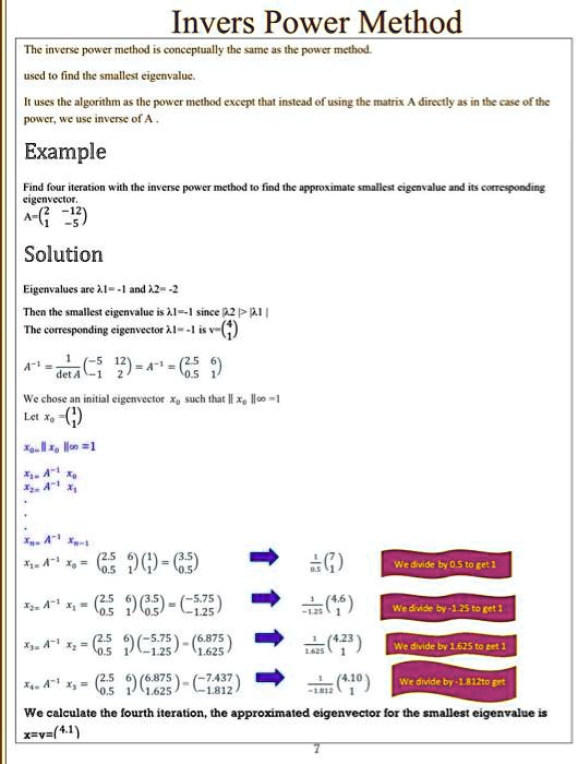
This image provides a worked example of the Inverse Power Method. It starts with a 2x2 matrix A, calculates its inverse A⁻¹, chooses an initial vector x₀, and performs four iterations. In each step, the next vector is calculated by multiplying A⁻¹ by the previous vector. The result is then normalized (by factoring out the bottom component) to prepare for the next iteration. The sequence of vectors converges toward the eigenvector associated with the smallest eigenvalue of A.

In this example, the iterations produce the following sequence of (un-normalized) vectors:

x_{1} = (3.5 0.5), x_{2} = (- 5.75 - 1.25), x_{3} = (6.875 1.625), x_{4} = (- 7.437 - 1.812)

After normalization (making the bottom component 1), the eigenvector approximations are:

(71) \to (4.6 1) \to (4.23 1) \to (4.10 1)

The sequence is clearly converging toward the exact eigenvector, which is $(41)$ .

As shown in the video LINK, once you have a good approximation of the eigenvector $x$ , you can find the corresponding eigenvalue $λ$ by computing $A x$ and finding the factor $λ$ such that $A x = λ x$ . Alternatively, you can take the reciprocal of the normalizing factor from the final iteration of the Inverse Power Method itself.

Conclusion

In this lesson, we have extended our knowledge of the Power Method to find not just the largest, but also the smallest eigenvalue of a matrix.

Here are the key takeaways:

The Inverse Power Method is simply the Power Method applied to the inverse of a matrix, $A^{- 1}$ .
It works because the eigenvalues of $A^{- 1}$ are the reciprocals of the eigenvalues of $A$ . Thus, the smallest eigenvalue of $A$ corresponds to the dominant eigenvalue of $A^{- 1}$ .
The process involves calculating $A^{- 1}$ , iterating multiplication and normalization to find the dominant eigenpair of $A^{- 1}$ , and then taking the reciprocal of the resulting eigenvalue to get $λ_{min}$ of the original matrix $A$ .

We can now find the eigenvalues at both extremes of the spectrum. But what if we need an eigenvalue that lies somewhere in the middle, or one that is closest to a specific value of interest? In our next lesson, we will explore the Shifted Inverse Power Method, a powerful extension that allows us to do just that.

Recommended resources

The Principle: Inverting the Problem

The Inverse Power Method Algorithm

A Hand-Calculated Example

Conclusion