Analyzing Algorithm Complexity

1. Why We Need Asymptotic Analysis

When we analyze an algorithm, we don't care about the exact number of seconds it takes to run. That number depends on the programming language, the hardware, the operating system, and other external factors. Instead, we want to understand how the algorithm's resource usage (like time or memory) changes as the size of the input, which we'll call $n$, gets larger.

Asymptotic analysis allows us to do this by focusing on the "growth rate" of the function that describes the algorithm's performance. We simplify the analysis by ignoring constant factors and lower-order terms, because as $n$ becomes very large, these details become insignificant.

For a high-level introduction to this idea, please watch the beginning of the following video.

2. The Three Core Notations: O, Ω, and Θ

Asymptotic analysis uses three primary notations to describe the bounds of an algorithm's performance.

a) Big O Notation (O): The Upper Bound

Big O is the most common notation you'll encounter. It describes an upper bound on the growth rate of a function. In simpler terms, it provides a worst-case scenario: an algorithm will perform at least as well as its Big O complexity.

Formal Definition:
A function $f(n)$ is in $O(g(n))$ if there exist positive constants $c$ and $n_0$ such that for all $n\ge n_0$, the following condition holds:
$f(n)\le c\cdot g(n)$
Here:

• $f(n)$ is the function representing your algorithm's actual runtime.
• $g(n)$ is a simpler function that provides an upper bound (e.g., $n^2$, $n\log n$).
• $n_0$ is the input size after which the upper bound holds true.
• $c$ is a constant factor that allows us to scale $g(n)$ to make the inequality true.

The key insight is that we can always find some constant c that makes the bound work for sufficiently large n. This is why we can ignore constants (e.g., $O(2n)$ is the same as $O(n)$) and lower-order terms (e.g., $O(n^2+n)$ simplifies to $O(n^2)$).

b) Big Omega Notation (Ω): The Lower Bound

Big Omega describes a lower bound. It provides a best-case scenario: an algorithm will take at least this long to run.

Formal Definition:
A function $f(n)$ is in $\Omega (g(n))$ if there exist positive constants $c$ and $n_0$ such that for all $n\ge n_0$:
$f(n)\ge c\cdot g(n)$

c) Big Theta Notation (Θ): The Tight Bound

Big Theta describes a tight bound. This is the most precise description, as it means the algorithm's growth rate is bounded both from above and below by the same function.

Formal Definition:
A function $f(n)$ is in $\Theta (g(n))$ if it is in both $O(g(n))$ and $\Omega (g(n))$. This means there exist positive constants $c_1$, $c_2$, and $n_0$ such that for all $n\ge n_0$:
$c_1\cdot g(n)\le f(n)\le c_2\cdot g(n)$

To solidify your understanding of these three notations with clear, visual examples and mathematical rigor, the next segment of the video is highly recommended.

For an additional, text-based reference on the formal definitions, you can review the following resource.

3. Analyzing Algorithm Complexity in Practice

Now let's apply this theory to real code. We will analyze the complexity of both iterative and recursive algorithms.

Analyzing Iterative Algorithms

For iterative code, we typically count the number of operations performed in relation to the input size n.

• O(1) (Constant Time): The number of operations does not depend on the input size. Examples include accessing an array element by index or performing a single arithmetic operation.

  def get_first_element(items):
      return items[0] # One operation, regardless of len(items)
  

• O(n) (Linear Time): The number of operations grows linearly with the input size. A common example is a single loop iterating through all n elements of a list.

  def find_max(items):
      max_val = items[0]
      for item in items: # Loop runs n times
          if item > max_val:
              max_val = item
      return max_val
  

• O(n^2) (Quadratic Time): The number of operations is proportional to the square of the input size. This often occurs with nested loops where both loops iterate up to n.

  def find_duplicates(items):
      for i in range(len(items)): # Outer loop runs n times
          for j in range(len(items)): # Inner loop runs n times
              if i != j and items[i] == items[j]:
                  return True # n*n = n^2 operations in the worst case
      return False
  

• O(log n) (Logarithmic Time): The number of operations grows very slowly as n increases. These algorithms typically reduce the problem size by a constant factor (e.g., by half) at each step. Binary search is the classic example.

The following video provides a practical, interview-focused walkthrough of these common complexities and more.

For further reading and more code examples, you can consult this guide.

Analyzing Recursive Algorithms

Analyzing recursion can be trickier. We need to define a recurrence relation that describes the runtime. A recurrence relation for a function $T(n)$ defines it in terms of its value on smaller inputs.

For a recursive algorithm, the time complexity $T(n)$ is typically the sum of:

1. The time it takes to do the work inside the current function call (e.g., comparisons, arithmetic).
2. The time it takes for all the recursive calls it makes.

Let's take a factorial function as an example:

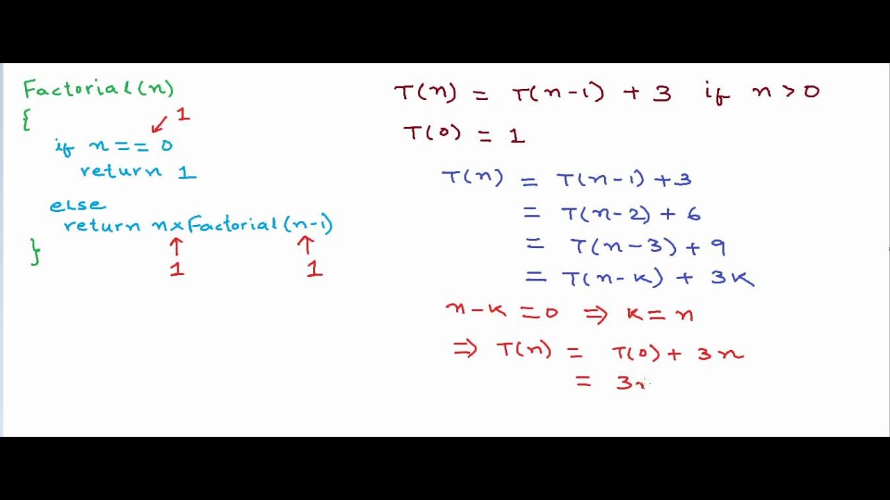
As you can see, the recurrence is T(n) = T(n-1) + 3. This is because each call does a constant amount of work (the check, multiplication, and return) and then calls itself on an input of size n-1. Solving this recurrence shows that the complexity is O(n).

A more complex example is the classic recursive Fibonacci function:

def fibonacci(n):
    if n <= 1:
        return n
    return fibonacci(n-1) + fibonacci(n-2) # Two recursive calls

The recurrence relation for this is $T(n)=T(n-1)+T(n-2)+c$. Because each call branches into two more calls, this leads to an exponential number of operations, resulting in a time complexity of $O(2^n)$. We will explore how to solve these recurrences more formally in a future lesson.

def my_function(n):
    i = 1
    count = 0
    while i < n:
        i = i * 2
        count += 1
    return count

Key Takeaways

• Asymptotic analysis describes how an algorithm's performance scales with input size n, ignoring constants and lower-order terms.
• Big O ($O$) provides an upper bound (worst-case).
• Big Omega ($\Omega$) provides a lower bound (best-case).
• Big Theta ($\Theta$) provides a tight bound (exact growth rate).
• For iterative code, complexity is found by analyzing loops. A single loop is often $O(n)$, nested loops can be $O(n^2)$, and algorithms that halve the input are often $O(\log n)$.
• For recursive code, complexity is described by a recurrence relation, which depends on the number of recursive calls and the work done at each step.

Next Steps

Excellent work on completing this foundational lesson. You now have the essential vocabulary and analytical tools to discuss algorithm efficiency.

In the next lesson, we will build directly on this by learning to differentiate between best, average, and worst-case complexities. We will see how a single algorithm can have different Big O complexities depending on the structure of its input data.