Hello! Welcome to your seventh lesson in the "Foundations of Algorithmic Analysis" module.
In our last lesson on binary search, we saw how a clever algorithm could reduce search time from linear O(n) to logarithmic O(log n). However, this came with a precondition: the array must be sorted, an operation that costs O(n log n) time. This raises a fundamental question: could we have used a different approach, like a hash map, to get O(1) average search time at the cost of O(n) memory?
This brings us to the core of today's lesson. Our learning outcome is to compare time-space trade-offs in algorithm design decisions. This isn't just about finding a solution; it's about evaluating multiple valid solutions and justifying your choice. For a senior developer like yourself, articulating these trade-offs is a key differentiator in high-level technical interviews, as it demonstrates architectural thinking.
We will explore how you can often make an algorithm faster by using more memory, or more memory-efficient by accepting a slower runtime.
1. The Fundamental Principle: Time vs. Space
At its heart, the time-space trade-off is a balancing act. In algorithm design, you are often faced with a choice:
- Optimize for Time: Pre-calculate and store results in memory (caching/memoization) to avoid re-computing them later. This speeds up execution but consumes more space.
- Optimize for Space: Re-calculate values on the fly as needed. This saves memory but can lead to slower execution times.

To formalize this concept, let's turn to a more academic resource.
ALGORITHMS AND COMPLEXITY ANALYSIS
The following text from a guide on complexity analysis provides a structured overview of this trade-off, using examples like Dynamic Programming and Hash Tables to illustrate the concept.
Please read 'Chapter Two: Time and Space Trade-offs', starting from the section 'Exploring the Trade-offs between Time and Space...' and continuing through to 'Memory vs. Computation'. Focus on the definitions and the examples given for Dynamic Programming, Merge Sort, and Hash Tables.
2. Case Study: Optimizing Fibonacci Numbers
The Fibonacci sequence is the classic example used to demonstrate time-space trade-offs. The n-th Fibonacci number is defined as fib(n) = fib(n-1) + fib(n-2), with fib(0) = 0 and fib(1) = 1.
Step 1: The Naive (and Slow) Recursive Approach
A direct translation of the definition into a recursive function is straightforward, but it's catastrophically inefficient.
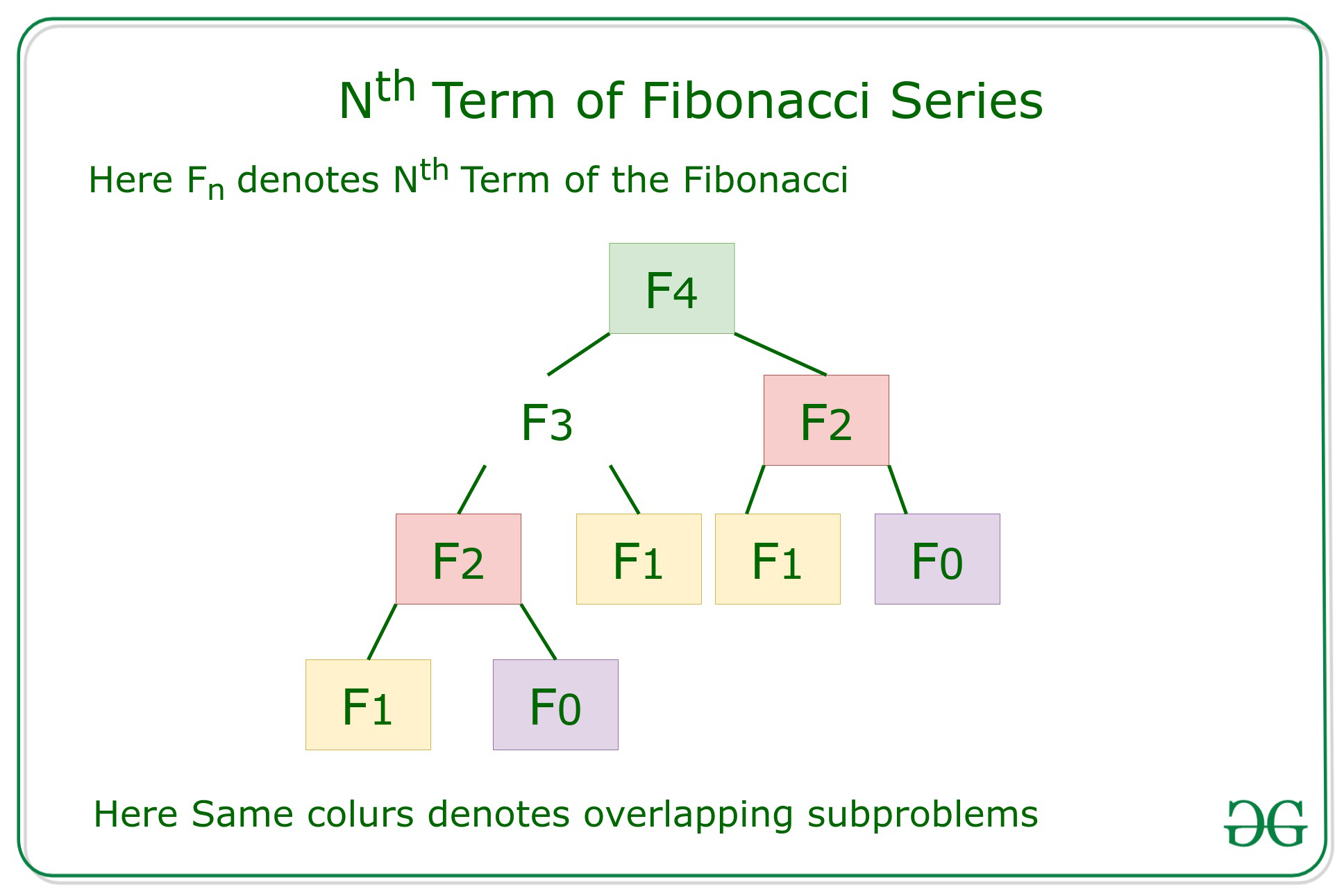
The video below explains why this approach has an exponential time complexity of O(2^n).
Algorithms: Memoization and Dynamic Programming
This video from HackerRank clearly illustrates the problem with the naive recursive solution for Fibonacci.
Watch from 00:33 to 01:59 to understand why the time complexity is exponential. Then, watch from 02:52 to 04:18, where the space complexity is discussed. Note the important distinction: even with exponential computations, the maximum depth of the call stack at any one time is O(n), so the space complexity is linear, not exponential.
Step 2: Trading Space for Time with Memoization
The inefficiency comes from re-calculating the same values. The solution? Memoization. We use a cache (like a hash map or an array) to store the results of function calls. Before computing fib(k), we first check if the result is already in our cache.
This is a direct time-space trade-off: we use extra space for the cache to achieve a massive speedup.
Dynamic Programming - Top Down Memoization & Bottom Up Tabulation - DSA Course in Python Lecture 15
This next video provides a fantastic, step-by-step walkthrough of the entire optimization process, from the naive solution all the way to a space-optimized one.
Watch from 02:41 to 13:07. This covers both the naive recursive approach and its optimization using memoization (top-down dynamic programming). Pay close attention to how the recursion tree is 'pruned' by the cache, drastically reducing the number of calls. The analysis of the new O(n) time and O(n) space complexity is key.
By using O(n) space for the cache, we reduced the time complexity from O(2^n) to a much more manageable O(n). This is a huge win and a common pattern in dynamic programming.
Step 3: Optimizing Space Back Down
Can we do better? Sometimes, after optimizing for time, we can find clever ways to reduce our space overhead. For Fibonacci, notice that to calculate fib(i), you only need the previous two values, fib(i-1) and fib(i-2). We don't need to store the entire sequence.
This leads to a "bottom-up" or tabulation approach that can be implemented with constant space.
Dynamic Programming - Top Down Memoization & Bottom Up Tabulation - DSA Course in Python Lecture 15
Let's continue with the same video to see how to optimize the space complexity.
Watch from 13:07 to 20:08. This section first explains the bottom-up approach with an O(n) space array (tabulation), and then shows the final optimization to an O(1) space solution using just two variables. This completes the full story of the time-space trade-off for this problem.
Fibonacci Optimization Summary:
| Approach | Time Complexity | Space Complexity | Trade-off |
|---|---|---|---|
| Naive Recursion | O(2^n) |
O(n) |
Base case, very slow. |
| Memoization (Top-Down) | O(n) |
O(n) |
Space for Time: Drastically faster. |
| Tabulation (Bottom-Up) | O(n) |
O(n) |
Avoids recursion overhead. |
| Space-Optimized (Bottom-Up) | O(n) |
O(1) |
Best of Both: Optimal time and space. |
3. Common Interview Patterns and Their Trade-offs
The ability to analyze these trade-offs is not limited to dynamic programming. It applies across all algorithmic patterns. Being able to discuss these options is crucial for your interviews.
The following document, "Coding Interview Prep," is an excellent resource that systematically discusses trade-offs for many common patterns. We won't read it all, but we will use it as a reference to highlight a few key examples.
Coding Interview Prep Chapter 1: Introduction
This guide is structured around discussing trade-offs, which is exactly our focus. We will refer to specific examples from it.
You don't need to read this now, but I want to point out its philosophy, which you should adopt: for each problem, explore brute-force solutions, optimized approaches, and the trade-offs between them (time, space, readability). This is the mindset of a top-tier candidate.
Here are some classic trade-off scenarios you should be ready to discuss:
| Problem Scenario | Approach A (Space-Heavy) | Approach B (Time-Heavy/Algorithm-Heavy) | Discussion Points |
|---|---|---|---|
| Finding Pairs (e.g., Two Sum) | Hash Map: O(n) Time, O(n) Space | Sort + Two Pointers: O(n log n) Time, O(1) Space (if in-place sort allowed) | If memory is no issue, the hash map is faster. If you cannot use extra space or the input is already sorted, the two-pointer approach is better. This is a classic interview question. (See LINK, section on "Two Pointers"). |
| Detecting Cycles (e.g., Linked List) | Hash Set: O(n) Time, O(n) Space | Floyd's Algorithm (Fast/Slow Pointers): O(n) Time, O(1) Space | Both are linear time, but Floyd's algorithm achieves this with constant space through a more complex pointer manipulation logic. If space is at a premium, Floyd's is superior. (See LINK, section on "Fast & Slow Pointers"). |
| Tree/Graph Traversal | BFS (Breadth-First Search): O(V+E) Time, O(W) Space (W = max width) | DFS (Depth-First Search): O(V+E) Time, O(H) Space (H = max height/depth) | The space trade-off depends on the graph's shape. For wide, shallow graphs, DFS is more space-efficient. For narrow, deep graphs, BFS is better. DFS can also cause stack overflow if not implemented iteratively. (See LINK, section on "Tree Traversal"). |
| Top K Elements | Sort: O(n log n) Time, O(1) Space | Min-Heap (Priority Queue): O(n log k) Time, O(k) Space | The heap approach is much faster if k is small compared to n, but it requires extra space. This is a common pattern for problems involving leaderboards or frequent items. (See LINK, section on "Heap and Priority Queue"). |
Test your understanding!
You are tasked with finding duplicate numbers in a large read-only file of n integers. The file is 100 GB, but you only have 1 GB of RAM. The numbers are within the range [1, n].
Which of the following approaches is most viable, and why, considering the time-space trade-offs?
- Hash Set: Iterate through the numbers, adding each to a hash set. If a number is already in the set, it's a duplicate.
- Sorting: Load the numbers into an array, sort it, and then iterate through to find adjacent duplicates.
- Cyclic Sort: Since the numbers are in the range
[1, n], you can use the cyclic sort algorithm to place each number at its correct index, identifying duplicates in the process.
Show answer
The most viable approach is not directly listed, highlighting the need to think creatively about constraints. Let's analyze the given options:
- 1. Hash Set: An
O(n)time andO(n)space solution. Sincenis large enough to create a 100 GB file, the hash set would also require tens of gigabytes of memory, far exceeding the 1 GB RAM limit. This is not viable. - 2. Sorting: An
O(n log n)time solution. Similar to the hash set, loading the entire 100 GB file into memory to sort is impossible with only 1 GB of RAM. While external sorting is a technique for this, it's complex and much slower. - 3. Cyclic Sort: An
O(n)time andO(1)space algorithm if you can modify the array in-place. However, the file is read-only, and even if it weren't, you can't load it all into memory.
So, what's the trade-off? You have a severe space constraint. This forces you to trade away the simplicity of in-memory algorithms for an approach that works with the given constraints.
A viable approach would be a variation of option 1 that uses disk space. You could read the file in chunks that fit into memory (e.g., 500 MB chunks). For each number in the chunk, you could hash it to determine which of, say, 200 "bucket" files on disk it belongs to. After one pass, you'd have 200 smaller files (around 500 MB each). Now, you can process each bucket file one by one. Since all numbers with the same value are guaranteed to be in the same bucket, you can load one bucket file into memory and use a hash set to find duplicates within that smaller set. This is a classic external memory algorithm strategy. It trades much higher I/O time (reading and writing the entire dataset multiple times) for manageable memory usage.
Conclusion
Understanding time-space trade-offs is about moving beyond "correct" and into "optimal for the given constraints." It is a conversation about design choices, and demonstrating this thought process is what separates good engineers from great ones in an interview setting.
Key Takeaways:
- Algorithms often present a choice between faster execution (time) and lower memory consumption (space).
- Caching/Memoization is a primary technique to trade space for significant time improvements, especially when dealing with overlapping subproblems.
- Conversely, analyzing memory access patterns can sometimes lead to space optimizations, reducing memory from
O(n)toO(1)while maintaining optimal time. - Being familiar with the trade-offs of common data structures (Hash Maps, Heaps) and algorithms (Sorting, Two Pointers, BFS/DFS) is essential for making informed design decisions.
In our next lesson, we will wrap up this foundational module by exploring bit manipulation. These are low-level techniques that operate directly on the binary representation of numbers, often leading to solutions with exceptional time and space efficiency.