Radial Probability and Most Probable Distance

Introduction

In our last lesson, we saw how the quantum numbers $n$ and $l$ give rise to the beautiful and complex shapes of atomic orbitals by defining their nodal structures. We ended on a subtle but profound point: for an s-orbital, while the density of the electron cloud ( $Ψ^{2}$ ) is highest right at the nucleus, this might not be where the electron is most likely to be found.

This lesson confronts that apparent paradox head-on. Our goal is to interpret the radial probability distribution, a concept that resolves this puzzle. We will explore why the most meaningful question isn't "At what point is the electron?" but rather "At what distance from the nucleus is the electron most likely to be?" By the end, you will be able to explain precisely why the electron in a hydrogen atom has a most probable, non-zero distance from the nucleus, a result that beautifully merges the wave nature of the electron with the simple geometry of space.

The Paradox: High Density at the Center, but the Electron is Elsewhere

Your classical intuition, grounded in electrostatics, might suggest the electron should be found at the nucleus, where the attractive force from the proton is strongest. The quantum mechanical probability density, $Ψ^{2}$ , partly agrees: for a 1s orbital, its value is maximal at $r = 0$ . So, why isn't the most probable location the nucleus itself?

The reason lies in the distinction between the probability at a point and the probability within a region. The volume of a single point is zero. It's more fruitful to ask: what is the total probability of finding the electron within a thin spherical shell at a distance $r$ from the nucleus?

Two competing factors are at play:

Probability Density ( $Ψ^{2}$ ): The likelihood of finding the electron per unit volume. For a 1s orbital, this decreases exponentially as you move away from the nucleus.
Volume of the Shell: The volume of a thin spherical shell is not constant; it grows as the radius increases. A shell with a large radius contains much more space than a shell with a small radius.

The actual probability of finding the electron at a distance $r$ is a product of these two competing trends. Let's build an intuition for this.

I finally understood orbital shapes intuitively! (My mind is blown)

This video from FloatHeadPhysics provides an excellent intuitive model for understanding how probability density and volume combine to create a 'probability map'.

Please watch from 06:00 to 12:06. Focus on these key ideas: The simulation (starting around 07:00) using dots to represent probability. Notice how the number of dots per shell first increases and then decreases, even though the dot density is highest at the center. The explanation (around 08:45) for why the center looks bright. This is a visual representation of the density-versus-total-probability paradox. The analogy of tracking a child's location (10:15) to reframe the concept of an orbital as a 'probability map' that answers "where is it most likely to be?", not "where is it?".

The Mathematical Resolution

The video provides a strong qualitative picture. Now, let's formalize it with the mathematics you appreciate. We want to find the probability, $d P$ , of finding the electron in an infinitesimally thin spherical shell of radius $r$ and thickness $d r$ .

This probability is the product of the probability density at that radius, $Ψ^{2} (r)$ , and the volume of that shell, $d V$ .

d P = Ψ^{2} (r) \cdot d V

The volume of a thin spherical shell is its surface area, $4 π r^{2}$ , multiplied by its thickness, $d r$ .

d V = 4 π r^{2} d r

Substituting this into our probability equation gives:

d P = Ψ^{2} (r) \cdot 4 π r^{2} d r

The term that multiplies $d r$ is what we're after. We call it the radial probability distribution function, $P (r)$ .

P (r) = 4 π r^{2} Ψ^{2} (r)

This function, $P (r)$ , gives the probability of finding the electron at a specific distance $r$ from the nucleus, summed over all possible directions.

The following video derives this function for the 1s orbital and shows what the resulting graph looks like.

Radial Probability Distribution of Hydrogen Atom in Ground State

Now that we have the conceptual framework, let's observe the formal derivation. This video by Andrey K rigorously constructs the radial probability distribution for the hydrogen ground state.

Please watch from 03:50 to 11:06. Concentrate on the logical steps: The conceptual leap from finding the probability at a point to finding it within a spherical shell of volume dV (starts around 05:25). The derivation of the volume element: dV = 4πr²dr (at 07:50). The definition of the radial probability distribution as the product of the squared wave function (density) and the surface area of the shell (geometry) (at 08:32). The final plot and its peak at the Bohr radius (r₀), identifying this as the most probable distance.

Visualizing the Competing Factors

The core insight is that $P (r)$ is a product of two functions: one that falls from a maximum at $r = 0$ (the $Ψ^{2}$ term) and one that rises from zero at $r = 0$ (the $4 π r^{2}$ term).

This image breaks down the relationship perfectly.

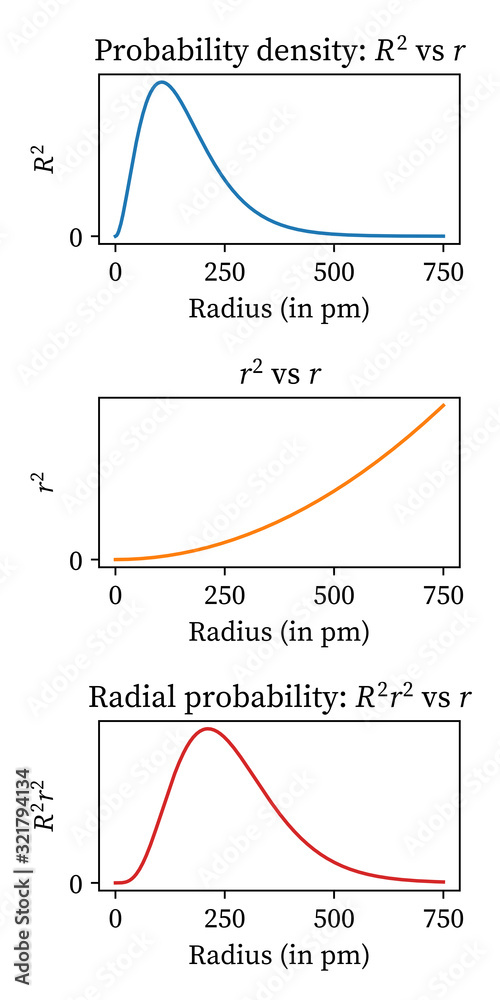
Radial Probability Distribution for an Electron — This figure deconstructs the radial probability distribution for a 1s orbital. The top graph shows the probability density ($R^2$, a component of $\Psi^2$), which peaks at the nucleus ($r=0$). The middle graph shows the $r^2$ term from the spherical shell's surface area, which is zero at the nucleus and grows quadratically. The bottom graph, the radial probability distribution ($P(r)$), is the product of the top two. The competition between them creates a peak at a non-zero radius, which is the most probable distance.

At $r = 0$ , the $4 π r^{2}$ term is zero, so the total probability $P (0)$ is zero. This is not a contradiction; it's a consequence of the geometry. Even if the probability density is high, the volume of the region you're considering is zero.

The following text provides a concise, rigorous explanation of this crucial point.

MITOCW Principles of Chemical Science Lecture Notes

To solidify our understanding, let's read a clear textual explanation from an MIT OpenCourseWare lecture note that directly addresses the common confusion about the probability at r=0.

Please read the initial sections of the document that define the radial probability distribution and analyze the graph for the 1s orbital. Look for the discussion starting around the definition of 'radial probability distribution'. Focus on two key points: The formula that combines probability density (\Psi^2) with the volume of the spherical shell (4\pi r^2 dr). The explicit explanation for why the probability is zero at r=0. The text stresses that this point is not a radial node but rather a mathematical consequence of multiplying by a volume term that is zero at the origin.

Radial Probability for Higher Energy Orbitals

This concept extends to all orbitals. The image below shows the radial probability distributions for the 1s, 2s, and 3s orbitals.

Electron Density, Wave Functions, and Radial Probability Distributions for s-Orbitals — This composite image shows: (a) the electron cloud representation, (b) the wave function $\Psi$, and (c) the radial probability distribution $P(r)$ for the 1s, 2s, and 3s orbitals. Notice how the most probable radius (the highest peak in graph c) moves further from the nucleus as the principal quantum number $n$ increases. Also, note the appearance of radial nodes (where $P(r) = 0$) for the 2s and 3s orbitals, matching our $n-l-1$ rule from the last lesson.

Guided Discovery

Let's use this concept to uncover a deeper layer of atomic structure. Consider the radial probability distributions for the 2s and 2p orbitals, which are often plotted on the same axes.

The 2p curve starts at zero, rises to a single maximum, and then tapers off. Its most probable radius is at 4 $a_{0}$ (where $a_{0}$ is the Bohr radius).
The 2s curve also starts at zero, but it has a small inner peak, dips to zero (a radial node), and then rises to a much larger peak before tapering off. Its most probable radius (the main, outer peak) is further out, at about 5.2 $a_{0}$ .

Now, let's analyze this:

Interpretation:
- The dip to zero in the 2s curve corresponds to the radial node we predicted ( $n - l - 1 = 2 - 0 - 1 = 1$ ). But what is the physical meaning of the small, inner peak for the 2s electron?
Comparison and the Concept of Penetration:
- The main peak for the 2s orbital is further out than the 2p's peak. This suggests a 2s orbital is, on average, "larger" than a 2p orbital.
- However, notice that the small inner peak of the 2s curve lies inside the 2p distribution. This means a 2s electron has a small but significant probability of being found very close to the nucleus, in a region where a 2p electron is never found. This effect is called penetration.
Probing Question (Foreshadowing):
- In a multi-electron atom, electrons in inner shells "shield" outer electrons from the full positive charge of the nucleus. Given that a 2s electron can penetrate this shield and get closer to the nucleus than a 2p electron can, what might you hypothesize about the relative energies of the 2s and 2p orbitals? Which electron would be more stabilized (lower in energy) by its interaction with the nucleus? Why?

Take your time to think through this. The answer is the key to understanding the layout of the entire periodic table.

Conclusion

Today, we resolved the paradox of the electron's location in an atom. We moved from the abstract idea of probability density to the more physically meaningful concept of radial probability distribution.

Key Takeaways:

The radial probability distribution $P (r)$ tells us the probability of finding an electron within a thin spherical shell at distance $r$ from the nucleus.
The most probable distance is non-zero because $P (r)$ is a product of two competing factors: the probability density ( $Ψ^{2}$ ), which is highest at the nucleus, and the shell volume ( $4 π r^{2}$ ), which is zero at the nucleus.
The point $r = 0$ on a radial probability graph is not a node; the probability is zero simply because the volume of a point-sized shell is zero.
As the principal quantum number $n$ increases, the most probable radius for the electron also increases, and radial nodes appear in accordance with the $n - l - 1$ rule.

We have now described the electron's "home" in space, defined by the quantum numbers $n$ , $l$ , and $m_{l}$ . However, the electron itself has one final, intrinsic property that is not related to its spatial wave function. In our next lesson, we will introduce the fourth and final quantum number—spin ( $m_{s}$ )—and see why this peculiar, non-classical property is the architectural key to building atoms with more than one electron.

Recommended resources