From Trajectories to Clouds: Interpreting the Wave Function ($\Psi$)

Introduction

In our last lesson, we dismantled the classical notion of an electron's path. We established that due to its wave nature, an electron exists as a wave packet, a fuzzy entity whose position and momentum are subject to the "unsharpness" of the Heisenberg Uncertainty Principle. This principle is not a limit on our instruments but a fundamental feature of reality. The idea of a deterministic, predictable trajectory is gone.

This leaves us with a profound question: If there's no trajectory, what is left? How do we describe the state of an electron in an atom? What, precisely, is the "wave" in wave-particle duality?

Today, we will answer that question by introducing the single most important concept in quantum mechanics: the wave function, symbolized by the Greek letter psi, $Ψ$ . Our goal is to interpret what this mathematical object represents. You will learn that $Ψ$ itself is not directly physical but is a probability amplitude. Its square, $∣Ψ ∣^{2}$ , gives us the probability of finding the electron at a particular point in space. This idea, known as the Born rule, marks the definitive shift from the clockwork universe of Newton to the probabilistic world of quantum mechanics.

The Problem of Interpretation: From Physical Wave to Probability Wave

When Erwin Schrödinger first formulated his famous wave equation, he had a natural, intuitive idea about what his wave function $Ψ$ represented. He imagined that the electron wasn't a point particle at all, but was literally "smeared out" in space, with the density of this "electron-stuff" at any point given by the value of $∣Ψ ∣^{2}$ at that point.

This was a beautiful, classical-like picture. However, it quickly ran into problems. For one, wave packets describing single particles can spread out over time, but we always detect electrons as whole, point-like entities. The "smeared-out" electron was never observed.

The correct, and much stranger, interpretation came from German physicist Max Born. He made a bold conceptual leap that defines quantum mechanics to this day.

Mysterious Quantum Rule Reconstructed From Scratch

To understand the context and gravity of Born's proposal, let's read an excerpt from an article in Quanta Magazine. It beautifully sets the stage, contrasting Schrödinger's initial intuition with Born's radical idea.

Please read the introduction and the first section, 'Where the Puzzle Is'. Focus on the distinction between Schrödinger's idea of a 'smeared-out' particle and Born's proposal of a 'wave of probability'. Note how Born's rule connects the abstract mathematics of \Psi to concrete, experimental predictions.

As the article states, Born's rule is the "crucial link between the abstract mathematical objects of quantum theory and the world of experience." It tells us that our theory doesn't predict what will happen, but rather the chances of various outcomes. The state of the electron is no longer a set of coordinates $(x, y, z)$ but a map of probabilities filling all of space.

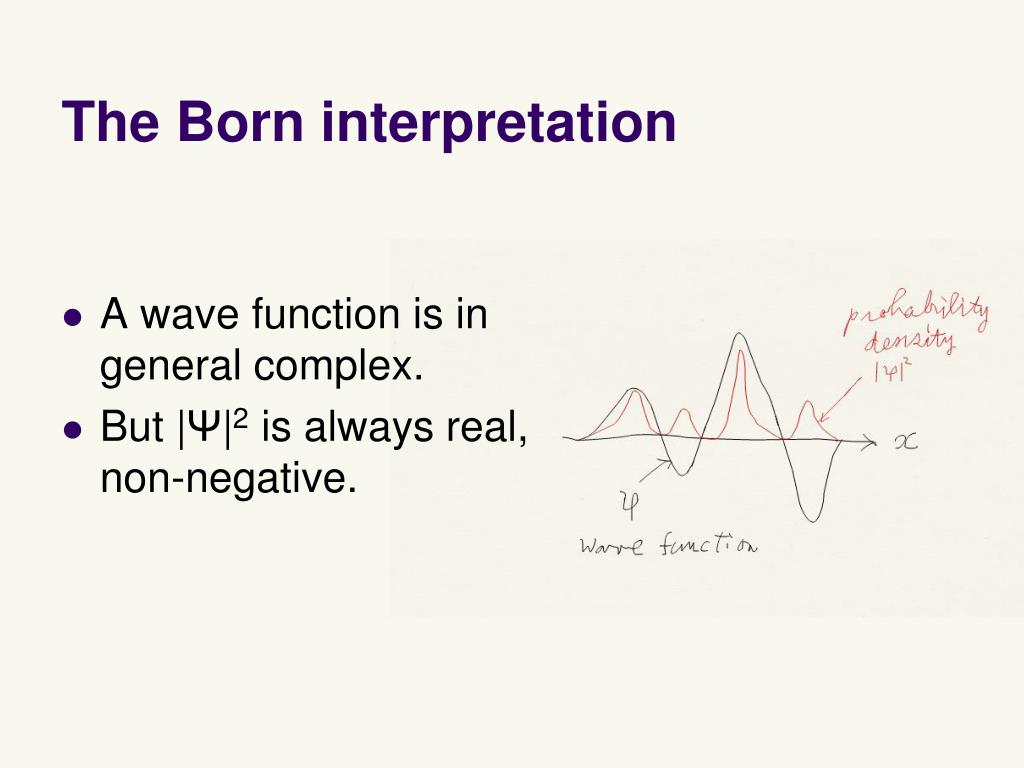
To visualize this, consider the following image.

The Born Interpretation of the Wave Function — This diagram illustrates the relationship between the wave function $\Psi$ and the probability density $|\Psi|^2$. The wave function (black curve) is a mathematical amplitude that can be positive or negative. The probability density (red curve), obtained by squaring the wave function, is always positive and represents the likelihood of finding the particle at a given position.

Why Amplitude Squared? The Logic of the Born Rule

You are a student who appreciates knowing the "why." So, why is the probability the square of the amplitude, $∣Ψ ∣^{2}$ , and not the amplitude $Ψ$ itself, or its absolute value $∣Ψ∣$ ? This is not an arbitrary choice. It is a deep mathematical necessity for building a consistent theory.

There are two immediate problems with using $Ψ$ directly:

Probability must be non-negative. As we can see in the image above, $Ψ$ can have negative values, which is nonsensical for a probability.
Interference. This is the crucial point. Individual probabilities do not interfere with each other. If there's a 50% chance of rain and a 20% chance of sun, these probabilities don't "cancel out." But waves do interfere. We need a mathematical object that can be added and subtracted (superposition) to produce interference patterns. Only after the interference has been calculated can we determine the final probability. The wave function $Ψ$ is that object.

The most rigorous way to see why it must be the square of the amplitude comes from demanding two very basic, logical conditions:

The total probability of finding the particle somewhere must be 1 (100%).
The description of the particle's state (the length of its state vector) shouldn't depend on the basis we use to describe it (e.g., energy basis vs. momentum basis).

Assuming these two simple ideas, it's possible to derive that the only consistent function relating the amplitude to probability is the square. The following video walks through this derivation. It is mathematically involved, but the conceptual path is elegant and provides exactly the kind of first-principles justification you seek.

Ch 8: Why is probability equal to amplitude squared? | Maths of Quantum Mechanics

The video 'Ch 8: Why is probability equal to amplitude squared?' from the channel Quantum Sense provides a brilliant derivation of the Born rule from first principles. It's challenging, but it will give you a profound appreciation for why the rule takes the form it does.

Watch from the beginning to 19:38. (00:19 - 02:45): The video starts by building the intuition that the size of the coefficient (the amplitude) along a certain state should relate to the probability of measuring that state. (02:45 - 07:17): It then demonstrates why a simpler rule, like taking the absolute value of the coefficient, leads to contradictions. It shows that this would make the 'length' of the quantum state change depending on what property you're trying to measure, which is logically inconsistent. (07:17 - 16:45): This is the heart of the derivation. By requiring the total probability to be 1 and the state's length to be constant, it derives a differential equation that the probability function must satisfy. The solution is that the probability must be proportional to the square of the coefficient. (16:45 - 19:38): Finally, it generalizes this to complex numbers (magnitude squared, |\Psi|^2) and explicitly connects the continuous coefficient function to the wave function. This directly addresses our learning outcome.

The essential takeaway is that the Born rule isn't an arbitrary postulate tacked onto quantum mechanics. It's the only rule that allows for a consistent probabilistic interpretation while preserving the fundamental structure of the theory.

From Trajectories to Probabilistic Clouds

With the Born rule, our picture of the atom changes forever. The electron is not in an orbit. The very word "orbital" is a misleading remnant of the Bohr model. A quantum orbital is not a path; it is a three-dimensional probability map, a standing wave of probability amplitude described by $Ψ$ .

I finally understood orbital shapes intuitively! (My mind is blown)

Let's build an intuition for what this 'probability map' looks like and what it means. The video 'I finally understood orbital shapes intuitively!' by FloatHeadPhysics uses excellent analogies to make this abstract concept concrete.

Please watch the following segments: (01:54 - 02:41): This section clearly states the modern view: the electron is a quantum particle, and the square of its wave function's amplitude gives the probability of finding it. (06:00 - 10:01): This segment simulates building the probability cloud for the ground state of hydrogen. It uses dots to represent probability and clarifies the common confusion about why the center looks bright even if the probability is highest at a non-zero radius. Pay close attention to the distinction between probability density and total radial probability. (10:01 - 12:06): This is a key analogy. It compares an orbital to a map of a child's likely locations. This perfectly captures the shift from a deterministic path ('orbit') to a probabilistic distribution ('orbital').

The language we use is important. To say an electron is "in" a 1s orbital does not mean it is moving on the surface of a sphere. It means its state is described by the 1s wave function, and the probability of finding it is highest at a certain radius and fades as you move away from the nucleus.

To reinforce this, the article below explicitly tackles the misconception of orbitals as orbits.

Models and Pictures of Atomic Wavefunctions

The webpage 'Models and Pictures of Atomic Wavefunctions' provides a sharp, technical clarification of these ideas.

Read Section 10, 'Quantum Mechanics versus Particle Mechanics'. It directly states that 'the spatial distribution of electrons is probabilistic, not deterministic. It is best visualized as a somewhat fluffy cloud.' It also emphasizes that 'orbitals are not orbits.'

Finally, let's look at a concrete example for the 1s and 2s orbitals.

Radial Wave Functions and Probability Densities for 1s and 2s Orbitals — This figure shows the radial wave function $\Psi(r)$ (top row) and the radial probability density $\Psi^2(r)$ (bottom row) for the 1s and 2s orbitals. Notice for the 2s orbital, the wave function passes through zero, creating a 'node'. This means there is a radius at which the probability of finding the electron is exactly zero—a result completely impossible in any classical model.

Guided Discovery

Let's probe the depths of these ideas.

Problem 1: The Revolutionary Leap

In your own words, explain the fundamental difference between Schrödinger's initial "smeared-out electron" interpretation of $∣Ψ ∣^{2}$ and Born's "probability density" interpretation. Why was Born's idea so much more radical and philosophically challenging?

Problem 2: Deconstructing a World

Let's conduct a thought experiment. Imagine a universe where the probability of finding a particle was given by $Ψ$ itself, not $∣Ψ ∣^{2}$ .
a) Look at the graph of the 2s wave function $Ψ (r)$ in the image above. What would this alternate rule imply about the "probability" of finding the electron in the region beyond the node? What fundamental property of probability is violated?
b) The essence of quantum mechanics is wave interference (e.g., the double-slit experiment). This relies on amplitudes adding or subtracting. If $Ψ$ directly represented probability, could two possibilities ever "cancel out" to zero probability? What does this tell you about the necessity of having an "amplitude" that is distinct from the probability itself?

Problem 3: Certainty and Uncertainty Revisited

In the previous lesson, we learned that a particle with a perfectly definite momentum ( $Δ p = 0$ ) is described by a pure sine wave that extends across all of space ( $Δ x \to \infty$ ).
a) A pure sine wave, like $sin (k x)$ , has a constant amplitude. What does Born's rule ( $P (x) = ∣Ψ (x) ∣^{2}$ ) tell you about the probability density of finding this particle at any given point $x$ ?
b) Based on your answer, how does the Born rule reinforce the conclusion of the Heisenberg Uncertainty Principle for this specific case?

Conclusion

Today, we have made the final and most crucial leap into the quantum worldview. We have replaced the deterministic mechanics of the past with a new, probabilistic framework.

Key Takeaways:

An electron's state is completely described by its wave function, $Ψ$ .
$Ψ$ is not a physical object, but a complex-valued probability amplitude. Its ability to be positive, negative, or complex is what allows for wave-like interference.
The connection to the real world is made through the Born rule: the probability density of finding a particle at a point is given by the square of the magnitude of the wave function at that point, $∣Ψ ∣^{2}$ .
This interpretation replaces the idea of a classical trajectory with a probabilistic cloud, or "orbital," which is a 3D map of the likelihood of locating the electron.

We are now equipped with the conceptual tools to understand the modern atom. We know that energy levels are quantized because of the standing wave condition, that position and momentum are inherently "unsharp," and that the electron's location is governed by probability.

But one big question remains: how do we find the specific wave function $Ψ$ for an electron in an atom? What rule dictates its shape and energy? In our next lesson, we will be introduced to the master equation of quantum mechanics—the Schrödinger equation. We will see that the stable states of an atom, our familiar s, p, and d orbitals, are nothing less than the fundamental solutions to this profound equation.