Heat Conduction in Cylinders and Spheres

1. Recap and Temperature Distribution

In the previous lesson, we treated hollow cylinders and spheres as thermal resistors. For a hollow cylinder of length $L$, inner radius $r_1$, outer radius $r_2$, and thermal conductivity $k$, we found the thermal resistance to be:

$R_{cyl}=\frac{\ln (r_2/r_1)}{2\pi kL}$

For a hollow sphere with the same parameters (except for length L):

$R_{sph}=\frac{r_2-r_1}{4\pi k{r}_1{r}_2}=\frac{1}{4\pi k}\left(\frac{1}{r_1}-\frac{1}{r_2}\right)$

While these are great for finding the total heat current $H=\Delta T/R$, we often need to know the temperature $T$ at some intermediate radius $r$ (where $r_1<r<r_2$). To do this, we need the temperature profile, $T(r)$.

Temperature Profile in a Hollow Cylinder

By integrating Fourier's Law but only up to an arbitrary radius $r$ instead of all the way to $r_2$, we can find the temperature distribution. For a hollow cylinder with inner surface at $T_1$ and outer surface at $T_2$, the temperature $T(r)$ is given by:

$\frac{T(r)-T_1}{T_2-T_1}=\frac{\ln (r/r_1)}{\ln (r_2/r_1)}$

Notice that the temperature does not vary linearly with radius, but logarithmically. This is a direct consequence of the area $A(r)=2\pi rL$ changing with the radius.

Temperature Profile in a Hollow Sphere

Similarly, for a hollow sphere, the temperature profile is:

$\frac{T(r)-T_1}{T_2-T_1}=\frac{\frac{1}{r_1}-\frac{1}{r}}{\frac{1}{r_1}-\frac{1}{r_2}}$

Here, the temperature varies inversely with the radius.

Let's see how these formulas are applied in a standard problem.

As you can see from the examples, the process is systematic: state the governing differential equation, integrate, apply boundary conditions, and solve for the constants to get the specific solution for $T(r)$. Then, use Fourier's law $H=-kA\frac{dT}{dr}$ to find the heat current.

2. Internal Heat Generation

A more advanced and common scenario in physics problems involves objects that generate their own thermal energy. A prime example is a wire carrying an electric current, where electrical energy is converted into heat due to resistance (Joule heating).

Let's consider a solid cylinder of radius $r_o$ and conductivity $k$, generating heat uniformly at a rate of ${\dot{e}}_{gen}$ per unit volume (units: W/m³). The outer surface is held at a constant temperature $T_s$.

In this case, the heat current $H$ is not constant along the radius. As we move from the center outwards, the heat current increases because more heat-generating volume is enclosed. We must return to the general heat conduction equation for a cylinder in steady state:

$\frac{1}{r}\frac{d}{dr}\left(r\frac{dT}{dr}\right)+\frac{{\dot{e}}_{gen}}{k}=0$

To solve this, we integrate twice. This process introduces two integration constants, which we must determine using two boundary conditions.

1. Surface Temperature: At the outer surface, the temperature is known: $T(r_o)=T_s$.
2. Symmetry at the Center: At the centerline ($r=0$), the temperature must be at a maximum due to symmetry. A smooth maximum implies that the temperature gradient is zero: ${\frac{dT}{dr}|}_{r=0}=0$. This is a crucial physical insight for solving such problems.

The solution from this derivation is a parabolic temperature profile:

$T(r)=T_s+\frac{{\dot{e}}_{gen}{r}_o^2}{4k}\left(1-\frac{r^2}{r_o^2}\right)$

This is a fundamental result. The temperature is maximum at the center ($r=0$) and decreases quadratically to $T_s$ at the surface.

3. Strategy for Composite Cylindrical/Spherical Systems

JEE Advanced problems often feature composite systems, such as an insulated pipe or a layered spherical container. Our thermal resistance analogy is still the most powerful tool here.

Consider a composite pipe made of two concentric layers (A and B), with heat flowing from a hot fluid inside to the ambient air outside.

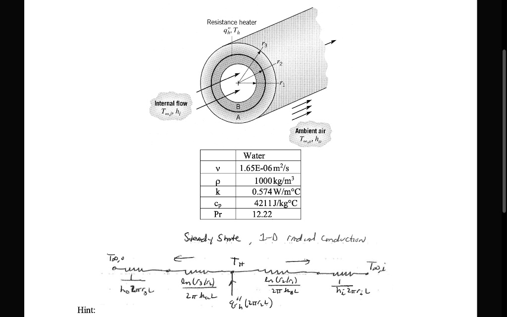
The total thermal resistance is the sum of the individual resistances in series:
$R_{total}=R_{conv,in}+R_{cond,A}+R_{cond,B}+R_{conv,out}$

We already know the conduction resistance formulas:

• $R_{cond,A}=\frac{\ln (r_2/r_1)}{2\pi k_{A}L}$
• $R_{cond,B}=\frac{\ln (r_3/r_2)}{2\pi k_{B}L}$

(We will cover the convection resistance terms, $R_{conv}=1/hA$, in a later module.)

If one of the layers involves heat generation, the problem becomes more complex. You cannot simply use the resistance formula for that layer. Instead, you must solve the heat equation within that layer and use the interface conditions (equal temperature and equal heat flux) to connect it to the adjacent layers.

This strategy of "divide and conquer" by solving for each region and then stitching the solutions together at the interfaces using boundary conditions is a powerful technique for many advanced physics problems.

Conclusion

In this lesson, we moved from deriving formulas to applying them to solve practical and complex problems involving cylindrical and spherical geometries.

Key Takeaways:

• The temperature distribution in a hollow cylinder (no heat generation) is logarithmic, while in a hollow sphere it varies as $1/r$.
• For a solid cylinder with uniform heat generation, the temperature profile is parabolic, with the maximum temperature at the center.
• The symmetry condition, $\frac{dT}{dr}=0$ at $r=0$, is a critical boundary condition for problems involving solid cylinders or spheres.
• Complex, multi-layered problems can be solved by breaking the system into individual components, finding the temperature profile for each, and connecting them by enforcing that temperature and heat flux are continuous at the interfaces.

Preview of the Next Lesson:
In all our problems so far, we have assumed that thermal conductivity $k$ is a constant. In reality, $k$ can change with temperature. In our next lesson, we will tackle the learning outcome: Tackle problems with temperature-dependent thermal conductivity. This will modify our integration step, as $k(T)$ will now be inside the integral with $dT$, but the fundamental principles of Fourier's law remain the same.