Understanding Common Complexity Classes

Visualizing Growth Rates

Let's start with a visual comparison. The "rate of growth" is what truly matters. As the input size (n) gets very large—which is what we care about in complexity analysis—the differences between these classes become dramatic.

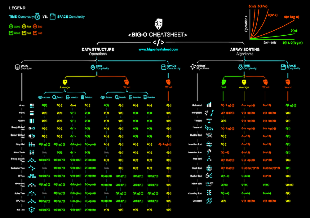
As you can see, the lines for O(n!), O(2^n), and O(n^2) curve upwards sharply, indicating they become slow very quickly. In contrast, O(log n) and O(1) are nearly flat, showing incredible efficiency even for massive inputs.

A Tour of the Complexity Classes

Let's explore these classes, generally from best to worst. The following video from NeetCode is an excellent, interview-focused guide that covers these concepts with clear examples. We will use it to structure our tour.

1. $O(1)$ — Constant Time

An algorithm with $O(1)$ complexity takes the same amount of time regardless of the input size. This is the ideal, most scalable performance.

• Examples: Accessing an array element by index (array[5]), pushing/popping from a stack, or simple arithmetic.

2. $O(\log n)$ — Logarithmic Time

This is a hallmark of highly efficient algorithms. If your algorithm has $O(\log n)$ complexity, it means that every time you double the input size, the number of operations only increases by one. This is typically achieved by repeatedly cutting the problem size in half.

• Classic Example: Binary search on a sorted array. You check the middle element and immediately discard half of the remaining elements.

This concept is crucial. Understanding why binary search is $O(\log n)$ is key.

To reinforce this, the following article provides a clear textual explanation with Java code, which should be familiar to you.

3. $O(n)$ — Linear Time

We covered this in the last lesson. The runtime grows proportionally to the input size. If you double the input, you double the work.

• Examples: Iterating through all elements of an array or linked list once.

4. $O(n\log n)$ — Log-Linear Time

This complexity class is very common and represents excellent performance for tasks that require comparing elements. It's slightly worse than $O(n)$ but significantly better than $O(n^2)$.

• Classic Examples: Efficient sorting algorithms like Merge Sort, Quick Sort, and Heap Sort. The log n part often comes from a "divide and conquer" strategy, and the n part comes from having to do that division n times or perform n operations at each level of division.

5. $O(n^2)$ — Quadratic Time

You're already familiar with this from nested loops. The runtime grows by the square of the input size. Doubling the input size quadruples the runtime. While acceptable for small n, it becomes problematic quickly.

• Examples: Simple sorting algorithms (Bubble Sort, Selection Sort), or iterating through all pairs of elements in a list using nested loops.

6. $O(2^n)$ and $O(n!)$ — Exponential and Factorial Time

These are among the worst-performing complexity classes. They are often associated with brute-force solutions that try every possible combination or permutation. An algorithm with this complexity is only practical for very small values of n.

• Examples: Generating all subsets of a set ($O(2^n)$), solving the traveling salesman problem via brute force ($O(n!)$).

The Big Picture: Why Comparison Matters

In an interview, you might first come up with an $O(n^2)$ solution. A great follow-up is to ask, "Can we do better?" This means trying to find an algorithm in a more efficient class, perhaps $O(n\log n)$ or even $O(n)$.

However, it's important to understand what "more efficient" really means. Big-O describes asymptotic behavior. An $O(\log n)$ algorithm is guaranteed to be faster than an $O(n)$ algorithm for a sufficiently large input n. For small inputs, the $O(n)$ algorithm might actually be faster due to smaller constant factors.

Let's test your understanding with a few practice questions.

Conclusion

In this lesson, we established a clear hierarchy of common complexity classes. Understanding this spectrum is fundamental to thinking like an effective programmer during a coding interview.

Key Takeaways:

• The Hierarchy of Efficiency (Best to Worst): $O(1)$ > $O(\log n)$ > $O(n)$ > $O(n\log n)$ > $O(n^2)$ > $O(n^3)$ > $O(2^n)$ > $O(n!)$.
• Logarithmic Time $O(\log n)$: Arises from algorithms that repeatedly cut the search space, typically by a constant fraction.
• Log-Linear Time $O(n\log n)$: Often the best possible for algorithms that must sort or perform complex comparisons.
• Asymptotic Behavior: Big-O compares algorithms based on their performance with large inputs. Your goal in an interview is almost always to find a solution in the best possible asymptotic complexity class.

In the next lesson, we will explore a related concept: the time-space tradeoff. You'll learn how you can sometimes achieve a faster time complexity by using more memory, a common strategic decision in algorithm design.