Data Storage Strategies for Machine Learning

The Database Landscape: SQL vs. NoSQL

The first major decision in designing a data layer is choosing a database model. Broadly, this choice falls into two camps: relational databases, queried with SQL, and a diverse group of non-relational databases, collectively known as NoSQL.

To begin, let's establish a high-level understanding of these database models and their trade-offs, with a focus on the practical considerations you'd face in a system design interview.

As the article highlights, the choice is not about finding the "best" database, but the most appropriate one for the job. Let's summarize the key characteristics:

• Relational (SQL) Databases (e.g., PostgreSQL, MySQL): These are the traditional workhorses. They organize data into tables with predefined schemas and enforce relationships and data integrity using foreign keys and constraints. Their key strength is ACID compliance (Atomicity, Consistency, Isolation, Durability), which guarantees that transactions are processed reliably. This is critical for systems where data integrity is paramount, like financial transactions or user account information. While sometimes criticized for scalability, modern SQL databases can scale to handle massive loads using techniques like read replicas and sharding.

• NoSQL Databases: This is a broad category of databases that moved away from the rigid, table-based structure of relational models. They generally offer more flexibility, horizontal scalability, and often prioritize performance and availability over the strict consistency guarantees of SQL. The main types we care about are:

  • Key-Value Stores (e.g., Redis, Amazon DynamoDB): The simplest NoSQL type. Data is stored as a collection of key-value pairs. They are incredibly fast for looking up a value when you know its key (GET user:123), but offer limited query capabilities beyond that. This makes them ideal for caching, session management, and, as we'll see, real-time feature serving.
  • Document Databases (e.g., MongoDB, Firestore): These store data in flexible, JSON-like documents. This is useful when your data structures are evolving or when different entities have different sets of attributes (e.g., user profiles). They model data in a way that is often more intuitive for developers.
  • Wide-Column Stores (e.g., Apache Cassandra, Google Bigtable): These databases store data in tables, but with a dynamic set of columns. They are optimized for huge datasets and very high write throughput. They are a common choice for time-series data, event logging, and large-scale analytics workloads.

A crucial concept related to database selection is the trade-off between normalization and denormalization.

• Normalization is the practice of organizing data to minimize redundancy (e.g., storing user information in a users table and referencing it by user_id in a posts table). This is the default in SQL and ensures data consistency.
• Denormalization is the practice of intentionally adding redundant data to improve read performance by avoiding costly joins (e.g., storing the username directly in the posts table). NoSQL databases often rely heavily on denormalization.

ML Access Patterns: The Dichotomy of Training and Serving

Now, let's connect these database concepts to the specific needs of machine learning systems. A defining characteristic of production ML is that it interacts with data in two fundamentally different ways:

1. For Model Training: We need to access large, historical datasets. We might need to scan terabytes of data spanning months or years to create a training set. This is a high-throughput, bulk read operation. Latency is not the primary concern; the ability to efficiently process huge volumes of data is.
2. For Online Inference: We need to fetch the most recent feature values for a single entity (like a user or a product) to feed into a live model. This must happen with very low latency—often in milliseconds. This is a high-concurrency, point-lookup operation.

No single database is optimized for both of these workloads. This leads to a common architectural pattern in ML systems: a dual-storage system often called a Feature Store. A feature store manages a collection of features and provides two distinct interfaces for accessing them: an offline store for training and an online store for serving.

Let's watch a segment that explains this dual requirement and the corresponding storage solutions.

As the video explains, a feature store's design directly reflects these two access patterns:

• The Offline Store: This component is built for bulk data access and historical analysis. It stores the complete history of feature values, often over long periods. The underlying technologies are typically data warehouses (like Google BigQuery, Amazon Redshift) or data lakes built on distributed file systems (like HDFS or Amazon S3) using columnar file formats (like Apache Parquet). These systems are optimized for large-scale analytical queries, exactly what's needed to build a training dataset.

• The Online Store: This component is built for speed. It holds only the latest value for each feature and is optimized for rapid key-based lookups. The technology of choice here is almost always a Key-Value Store like Redis or DynamoDB. When a prediction request comes in for user_id: 123, the model serving application queries the online store to get that user's latest features in milliseconds.

To explore this dual-layer architecture with some more specific technology examples, let's look at another resource.

Caching Strategies for Performance

The online store in a feature store is a specialized form of a cache. More generally, caching is one of the most important techniques for improving system performance and scalability. A cache is a high-speed data storage layer that stores a subset of data, typically transient, so that future requests for that data are served up faster than is possible by accessing the data's primary storage location.

By placing a cache in front of a slower database, you can significantly reduce latency for read-heavy workloads and decrease the load on your primary database. Key-value stores like Redis and Memcached are the standard technologies used for caching.

However, simply "adding a cache" isn't a complete design choice. You must also decide on a caching strategy that defines how and when data is written to and read from the cache. Let's review the most common patterns.

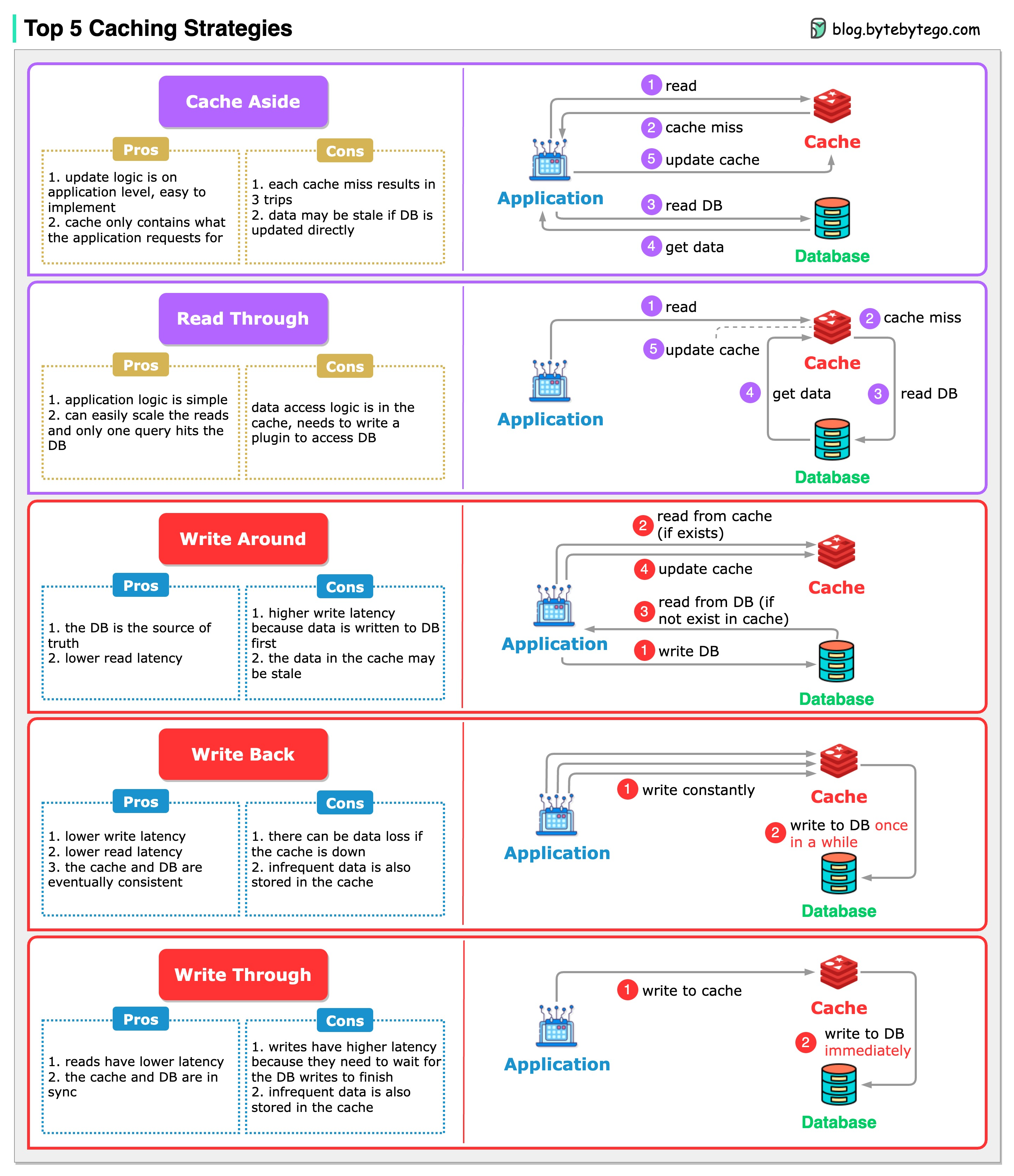
Let's walk through the strategies from the "Top 5 Caching Strategies" diagram:

1. Cache-Aside (or Lazy Loading): This is the most common strategy.

   • Read: The application first checks the cache. If the data is there (a cache hit), it's returned. If not (a cache miss), the application reads the data from the database, loads it into the cache, and then returns it.
   • Write: The application writes directly to the database.
   • Pros: Simple to implement, resilient to cache failures (the app can still get data from the DB).
   • Cons: Higher latency on the first read (the cache miss), and potential for stale data if the DB is updated directly by another service.

2. Read-Through: The cache itself handles the logic of fetching from the database.

   • Read: The application queries the cache. If it's a miss, the cache is responsible for fetching the data from the database, storing it, and returning it to the application.
   • Pros: Simplifies application code.
   • Cons: The cache needs a plugin or connector to talk to the database.

3. Write-Through: Writes go through the cache to the database.

   • Read: Same as Cache-Aside.
   • Write: The application writes to the cache, and the cache immediately writes to the database. The operation is only complete when both writes succeed.
   • Pros: Data in the cache and database is always consistent.
   • Cons: Higher write latency because you are writing to two systems synchronously.

4. Write-Back (or Write-Behind):

   • Read: Same as Cache-Aside.
   • Write: The application writes only to the cache, which immediately confirms the write. The cache then asynchronously writes the data to the database in the background after a delay.
   • Pros: Very low write latency. Excellent for write-heavy applications.
   • Cons: Risk of data loss if the cache fails before the data is persisted to the database.

5. Write-Around:

   • Read: Same as Cache-Aside.
   • Write: The application writes directly to the database, bypassing the cache entirely.
   • Pros: Reduces cache "churn" caused by writing data that isn't read immediately.
   • Cons: A read immediately after a write will be a cache miss, incurring higher latency. This is suitable for workloads like logging or analytics where data is written once and read infrequently.

Understanding these patterns allows you to make a much more nuanced and impressive recommendation in a design interview than simply saying "I'd add a cache."

Conclusion

In this lesson, we navigated the complex landscape of data storage, from foundational database models to specific caching patterns. You've learned how to map these technology choices to the unique demands of machine learning workflows.

Here are the key takeaways:

• SQL vs. NoSQL: The choice depends on your requirements for schema rigidity, data consistency, and query patterns. SQL databases offer strong consistency (ACID) and are a reliable default, while NoSQL databases provide flexibility and horizontal scalability for specific use cases (key-value, document, wide-column).
• ML's Dual Access Pattern: ML systems require both high-throughput bulk reads for training (the Offline Store) and low-latency point-in-time reads for inference (the Online Store).
• Feature Store Architecture: This dual need is commonly addressed with a hybrid architecture: data warehouses or data lakes (e.g., BigQuery, S3 with Parquet) for the offline store, and fast key-value stores (e.g., Redis) for the online store.
• Caching Strategies: Caching is critical for performance. The optimal strategy (e.g., Cache-Aside, Write-Through, Write-Back) depends on the trade-offs you're willing to make between read/write latency, data consistency, and implementation complexity.

We've now covered how to scale compute, organize application logic, and store data. You may have noticed that many of these choices, especially with distributed NoSQL databases and caching, involve trade-offs with data consistency. In our next lesson, we will formalize these trade-offs by exploring the CAP theorem, a fundamental principle that governs all distributed data systems.