In our last lesson, we established the static blueprint of a feature store, identifying its core components: the high-throughput offline store for training, the low-latency online store for serving, and the feature registry for metadata management. Now, we will bring this architecture to life by designing the dynamic data flows that populate these stores.
This lesson focuses on the learning outcome: Design data flows for feature computation, distinguishing between online and offline contexts. We will map out the journey of data from its raw state to a computed feature, ready for use. Understanding this distinction between batch (offline) and streaming (online) computation is not just a technical detail; it's a central theme in ML system design interviews, forcing a discussion of trade-offs between data freshness, computational cost, and implementation complexity. Your experience in data science means you're an expert in the what of feature engineering; this lesson will focus on the how at production scale.
The Core Dilemma: Batch vs. Real-Time
When designing a system that computes features, the first critical decision is whether to process data in large, scheduled batches or as a continuous, real-time stream. This choice impacts the entire architecture, from cost and complexity to the ultimate accuracy and responsiveness of your ML model.
A mock system design interview provides an excellent illustration of how to approach this trade-off.
Spotify ML Question - Design a Recommendation System (Full mock interview)
This video captures a mock interview for designing a recommendation system. The candidate's thought process is highly relevant to our topic.
Please watch the segment where the candidate discusses the cadence of recommendations, from batch versus real-time. Pay close attention to their reasoning around the trade-offs: a batch system is simpler and less compute-intensive, while a real-time system might offer better accuracy. This is the fundamental trade-off we will explore throughout this lesson.
As the video highlights, there isn't a single "correct" answer. Production systems often employ a hybrid approach, using different data flows for different types of features. Our feature store architecture is designed to accommodate exactly this hybrid model. Let's use the diagram below to visualize these parallel data flows.

The Offline Flow: Batch Feature Computation
The offline, or batch, data flow is the workhorse for generating the vast majority of features used in machine learning. It's designed for throughput and cost-efficiency over latency.
Purpose:
- Generating Training Data: To create large, historical datasets for training and retraining models.
- Computing Stable Features: To calculate features that change infrequently and don't require millisecond freshness for inference (e.g., a user's total number of purchases, a product's average rating over 30 days).
The Process:
This flow typically runs on a schedule (e.g., hourly or daily) and follows these steps:
- Source: A job orchestrator (like Apache Airflow) triggers a batch job.
- Extract & Transform: A batch processing engine, most commonly Apache Spark, reads large volumes of raw data from a data lake (e.g., Amazon S3) or a data warehouse (e.g., Snowflake, BigQuery).
- Compute: The Spark job applies the feature engineering logic—aggregations, encodings, etc.—to transform the raw data into feature values.
- Load: The resulting feature data, indexed by entity IDs and timestamps, is written into the offline store.
The following video provides a clear walkthrough of this batch ingestion process.
ML System Design: Feature Store
This video segment explains how batch processing systems are used to ingest features into a feature store from raw data sources.
Watch the portion on batch processing from the description of raw data sources to the end of the batch section. Notice the collaboration mentioned between data engineers, who manage the data infrastructure, and data scientists, who define the feature logic.
To make this more concrete, the article "Building Machine Learning Pipelines with the FTI Architecture" provides a simplified code-level view of this process.
Building Machine Learning Pipelines with the FTI ...
This article breaks down an ML pipeline into Feature, Training, and Inference stages. The "Feature Pipeline" section is a practical illustration of our offline flow.
Please read Step 1: Building the Feature Pipeline. Focus on the three sub-steps: Data Extraction: Reading data from a source (in this case, a SQL database). Feature Engineering: Applying transformations using pandas. In a large-scale system, this logic would run in a distributed framework like Spark. Storing Features: Defining the feature's schema and registering it with the feature store.
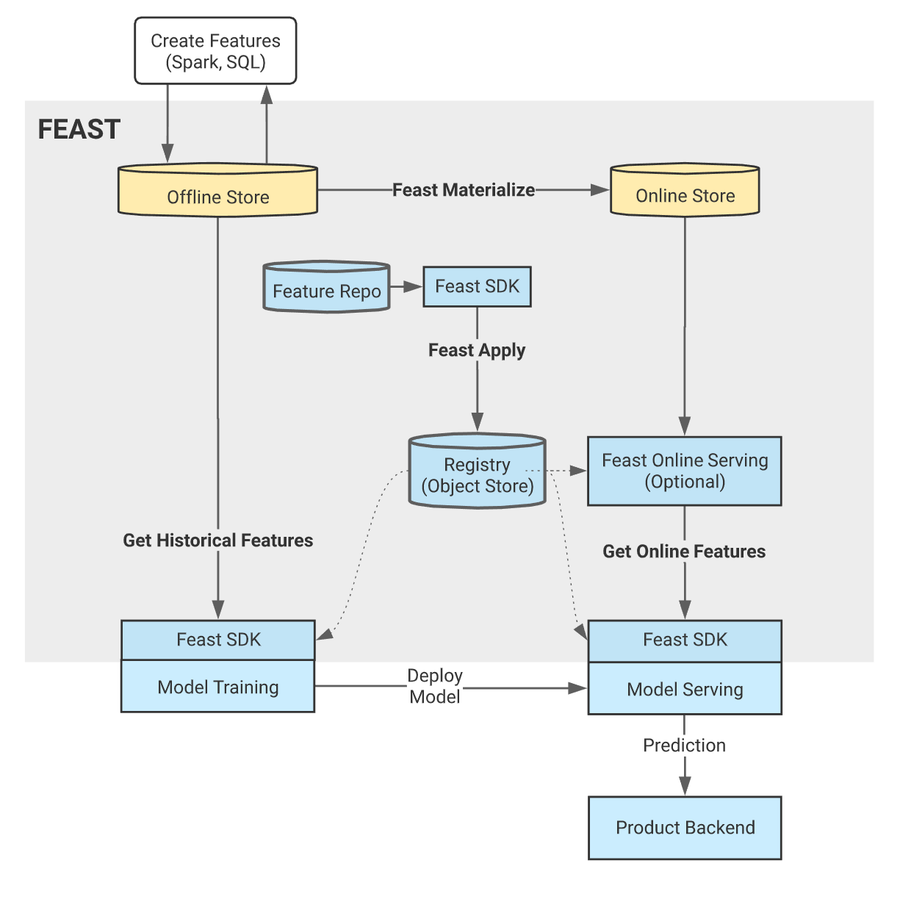
Materialization: From Offline to Online
After the batch job populates the offline store, there's one more crucial step. For the newly computed features to be available for low-latency inference, their latest values must be loaded into the online store. This process is called materialization. It's essentially a sync from the analytical offline store (like a data lake) to the operational online store (like Redis).
The architecture of Feast, an open-source feature store, illustrates this step perfectly.
The Online Flow: Streaming Feature Computation
While the batch flow is ideal for historical and slow-moving features, some use cases demand features that reflect events that happened just seconds ago. This is where the online, or streaming, data flow comes in.
Purpose:
- Real-time Features for Inference: To compute highly dynamic features that capture immediate user behavior or system state (e.g.,
number_of_clicks_in_last_minute,time_since_last_purchase).
The Process:
This flow processes data continuously as it arrives:
- Source: Real-time events (e.g., clicks, views, transactions) are published to a distributed message queue, like Apache Kafka. Each event is a small, structured message.
- Consume & Transform: A stream processing engine, such as Apache Flink or Spark Streaming, subscribes to the Kafka topic and consumes events as they are published.
- Compute: The engine performs stateful computations, often over time-based windows. For example, it can maintain a rolling count of clicks for each user over a 5-minute sliding window.
- Load: The computed feature values are written directly to the online store (e.g., Redis), overwriting the previous values. This makes them immediately available to the model serving API with very low latency.
This flow is elegantly explained in the "Preparing for ML Infra System Design Interviews" article.
Preparing for ML Infra System Design Interviews
This article provides an excellent, interview-focused breakdown of ML system components. The section on real-time generation is particularly relevant.
In the "Offline Path: Generate Data to Train Models" section, please read the part on real-time features. This passage clearly describes the canonical streaming architecture: using a messaging system like Kafka combined with a stream processor like Flink to compute features and write them to the feature store for serving.
Unifying the Flows
At the moment of a prediction request, the model serving system needs to assemble a complete feature vector for an entity. This vector is often a combination of features computed by both flows.
For instance, when a user requests a personalized feed, the system might fetch:
- Batch Features:
user_age_group,lifetime_purchase_count,preferred_product_category(computed daily). - Streaming Features:
in_session_click_count,time_since_last_activity(updated in real-time).
The model serving API queries the online store, which seamlessly provides the latest values for all these features, regardless of which flow computed them.
Modern feature platforms aim to provide a unified interface for this dual-path computation. An ML engineer can declaratively define a feature (e.g., "count of user clicks over 30 days"). The platform then automatically orchestrates both:
- A daily batch job to backfill the feature's historical values for training.
- A streaming job to incrementally update the feature's value in real-time as new clicks occur.
This abstraction significantly simplifies the process for data scientists, allowing them to focus on feature logic rather than the underlying data engineering.
Conclusion
In this lesson, we have animated our feature store architecture by designing the data flows that power it. You can now distinguish between the two primary modes of feature computation and articulate the design of each.
Key Takeaways:
- Feature computation is divided into two main data flows: offline (batch) and online (streaming).
- Offline flows are for throughput and cost-efficiency. They use batch engines like Spark on a schedule to process data at rest (from data lakes/warehouses), generating historical data for training and stable features for inference.
- Online flows are for freshness and low latency. They use stream processors like Flink to compute features from real-time event streams (from Kafka), providing up-to-the-second data for inference.
- Materialization is the critical process of moving the latest feature values computed offline into the online store to make them accessible for real-time serving.
- At inference time, a model's feature vector is often a composite of features derived from both batch and streaming pipelines.
We now understand how features are computed for training (via the offline flow) and serving (via both flows, accessed through the online store). However, a subtle but critical risk emerges: what if the feature logic in the batch pipeline is slightly different from the logic in the streaming pipeline? This can lead to a dangerous problem called training-serving skew. In our next lesson, we will design strategies to prevent training-serving skew, ensuring that the features our model sees in production are consistent with the features it was trained on.