DFA Computation Trace

The Intuition of a Computation

At its heart, a DFA's computation is a journey through its state diagram. The machine starts in the designated start state. It then reads the input string one symbol at a time from left to right. For each symbol, it follows the single, uniquely defined transition arrow from its current state to the next. When the string is exhausted, the journey ends. If the final state is an accepting state (a double circle), the string is accepted; otherwise, it is rejected.

Let's consider the following DFA as our example for this lesson:

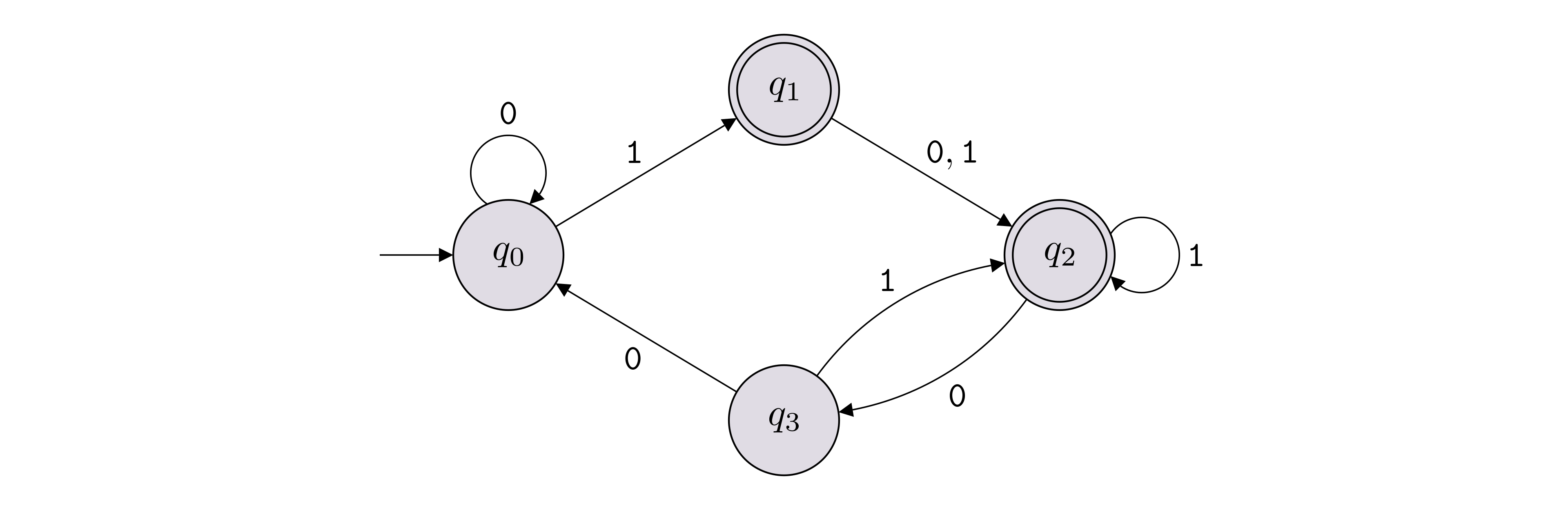
Let's trace the input string 101 on this machine intuitively:

1. Start: The machine begins at the start state, $q_0$.
2. Read 1: From state $q_0$, the transition for the symbol 1 leads to state $q_1$. The machine is now in state $q_1$.
3. Read 0: From state $q_1$, the transition for the symbol 0 leads to state $q_2$. The machine is now in state $q_2$.
4. Read 1: From state $q_2$, the transition for the symbol 1 leads back to state $q_2$ (a self-loop). The machine remains in state $q_2$.
5. End of string: We have processed all symbols. The machine's final state is $q_2$.

Since $q_2$ is in the set of accepting states $F=\{q_1,q_2\}$, we conclude that the DFA accepts the string 101. The sequence of states visited was $q_0\to q_1\to q_2\to q_2$.

This intuitive trace is useful, but for formal proofs and unambiguous definitions, we need to ground this process in mathematics.

Formalizing Computation: The Extended Transition Function

The transition function, $\delta :Q\times \Sigma \to Q$, is defined to handle only a single input symbol. To formalize computation over an entire string, we must extend it. We define the extended transition function, commonly denoted as $\hat{\delta }$ (pronounced "delta-hat"), which takes a state and a string as input and returns the state the machine is in after processing that string. Its signature is $\hat{\delta }:Q\times {\Sigma }^{\ast }\to Q$.

Given your background in mathematical proofs, you will find its inductive definition quite natural:

• Base Case: For the empty string $\epsilon$, no transitions occur. $$\hat{\delta }(q,\epsilon )=q$$
• Recursive Step: For any string $w\in {\Sigma }^{\ast }$ and any symbol $a\in \Sigma$, the string $wa$ is one symbol longer than $w$. We find the state after processing $w$, and then apply the standard transition $\delta$ for the final symbol $a$. $$\hat{\delta }(q,wa)=\delta (\hat{\delta }(q,w),a)$$

With this function, we can formally define acceptance. A DFA $M=(Q,\Sigma ,\delta ,q_0,F)$ accepts a string $w\in {\Sigma }^{\ast }$ if and only if $\hat{\delta }(q_0,w)\in F$.

To see a detailed walkthrough of this definition and a concrete example of its application, please watch the following video.

Let's apply this to our earlier trace of 101 on the example DFA. We want to compute $\hat{\delta }(q_0,101)$.

1. $\hat{\delta }(q_0,101)=\delta (\hat{\delta }(q_0,10),1)$
2. To solve this, we need $\hat{\delta }(q_0,10)$:
   $\hat{\delta }(q_0,10)=\delta (\hat{\delta }(q_0,1),0)$
3. And for that, we need $\hat{\delta }(q_0,1)$:
   $\hat{\delta }(q_0,1)=\delta (\hat{\delta }(q_0,\epsilon ),1)=\delta (q_0,1)=q_1$
4. Now we can substitute back into step 2:
   $\hat{\delta }(q_0,10)=\delta (q_1,0)=q_2$
5. Finally, we substitute back into step 1:
   $\hat{\delta }(q_0,101)=\delta (q_2,1)=q_2$

The result is $q_2$. Since $q_2\in F$, the string 101 is accepted, matching our intuitive trace.

An Alternative View: Sequences of Configurations

Another way to formalize computation is by describing it as a sequence of "snapshots" of the machine. Each snapshot is called a configuration and captures the machine's current state and the remaining portion of the input string. A configuration is typically written as a pair $(q,w)$, where $q$ is the current state and $w$ is the unread part of the input.

The process of moving from one configuration to the next is defined by the yields relation, denoted by the $⊢$ symbol.
We say $(q,aw)⊢(p,w)$ if $\delta (q,a)=p$. This means that if the machine is in state $q$ with aw left to read, it can take one step to be in state $p$ with just w left to read.

A full computation is a sequence of such steps. We use ${⊢}^{\ast }$ (the reflexive, transitive closure of $⊢$) to denote zero or more steps. A DFA accepts a string $w$ if the initial configuration yields a final configuration where the input is empty and the state is an accepting one. Formally:
$(q_0,w){⊢}^{\ast }(q_f,\epsilon )$ for some $q_f\in F$.

To explore these concepts in more detail, please consult the following resource.

The Computation Trace as a Sequence of States

Both the extended transition function and the sequence of configurations describe the same underlying phenomenon: the unique path of states the DFA takes for a given input. This path is the computation trace.

For an input string $w=w_1{w}_2...w_n$ of length $n$, the computation is a sequence of $n+1$ states, let's call it $s_0,s_1,...,s_n$, where:

1. $s_0=q_0$ (the computation starts in the start state).
2. $s_i=\delta (s_{i-1},w_i)$ for $i=1,...,n$ (each subsequent state is determined by the transition from the previous state on the corresponding input symbol).

The string $w$ is accepted if the final state in this sequence, $s_n$, is an accepting state.

It's important to recognize this as a sequence rather than a set of states. A state can be visited multiple times, and the order of visits is fundamental to the computation. The following video clarifies this distinction and provides another formal definition of a computation.

Conclusion

In this lesson, we have moved from the static definition of a DFA to its dynamic operation. We have meticulously defined what it means for a DFA to compute and to accept a string.

Here are the key takeaways:

• A DFA's computation is a step-by-step process of reading an input string and transitioning between states.
• This process can be formally described using the extended transition function, $\hat{\delta }$, which recursively determines the final state after processing an entire string.
• Alternatively, computation can be seen as a sequence of configurations, where the machine moves from one configuration to the next via the yields relation, $⊢$.
• The result of a computation on an input string $w$ is a unique trace, a sequence of states $s_0,s_1,...,s_n$.
• A string $w$ is accepted if and only if the final state in its computation trace, $s_n$, is an element of the DFA's set of accepting states, $F$.

Now that you can precisely trace a DFA's execution, you are ready for the next logical step. In our next lesson, we will shift from analyzing existing DFAs to designing new ones to recognize specific languages we want to capture.