From Logits to Binary Mask: Isolating Facial Features

From Raw Scores to Probabilities

A segmentation model like DeepLabV3 finishes its forward pass by producing a tensor of logits. For an input image of size $H\times W$, the output might be a tensor of shape $C\times H\times W$, where $C$ is the number of classes the model was trained to identify. A logit is simply the raw, unbounded numerical output of the network for a given pixel and class. It is not a probability; it can be any real number, from highly negative to highly positive.

To make sense of these values, we must convert them into probabilities. The method for doing this depends on whether we are solving a binary or a multi-class problem.

The Binary Case: Sigmoid Activation

For your project, the ultimate goal is to create a single mask that isolates the teeth. This is a classic binary segmentation problem: each pixel is either "teeth" (1) or "not-teeth" (0). In this scenario, the model would be configured to have a single output channel ($C=1$). The logit for each pixel then represents the model's confidence that the pixel belongs to the "teeth" class.

To convert this single logit per pixel into a probability, we use the sigmoid function.

The sigmoid function "squashes" any real-valued input $z$ (the logit) into a value between 0 and 1. A large positive logit results in a probability near 1, a large negative logit results in a probability near 0, and a logit of 0 results in a probability of 0.5.

From Probabilities to a Binary Mask

After applying the sigmoid function to the logit map, we have a probability map. This is a grayscale image where the intensity of each pixel (from 0.0 to 1.0) represents the model's probabilistic belief that the pixel belongs to the "teeth" class.

To get our final binary mask, we need to make a firm decision for each pixel. This is achieved through thresholding. The most common practice is to use a threshold of 0.5.

• If a pixel's probability is greater than 0.5, we classify it as foreground (teeth) and set its value in the mask to 1 (white).
• If a pixel's probability is less than or equal to 0.5, we classify it as background (not-teeth) and set its value to 0 (black).

The image below illustrates the effect of thresholding. While it shows different thresholding methods, the top row provides a good analogy for our process: an image with continuous values (like our probability map) is converted into a stark, binary image.

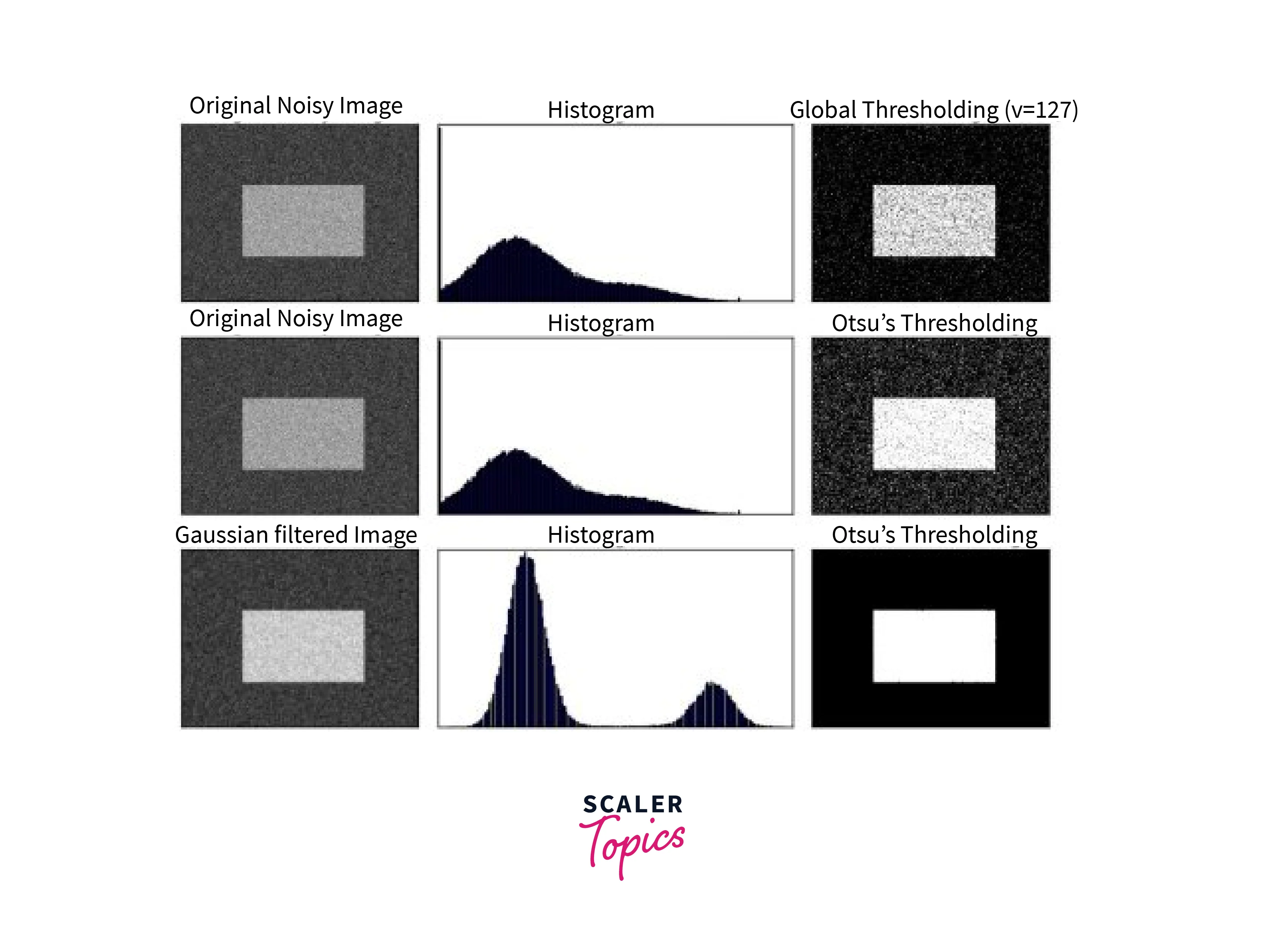
This entire process—from logits to a binary mask—can be expressed very concisely in code. You'll often see a line that looks like this in PyTorch:

mask = (torch.sigmoid(logits) > 0.5)

This single line performs the element-wise sigmoid activation on the raw logits and then the element-wise comparison against the 0.5 threshold, resulting in a boolean tensor that serves as our binary mask.

The Multi-Class to Binary Workflow

In many practical situations, you might use a powerful, pre-trained segmentation model that was trained on a dataset with many classes (e.g., skin, hair, lips, teeth, background). Your model's output would then be a logit tensor with multiple channels, one for each class ($C>2$). How do you get a binary "teeth" mask from this?

There are two common approaches.

1. Softmax and Argmax

First, you can apply the softmax function across the channel dimension. Unlike sigmoid which acts on each channel independently, softmax normalizes the logits for each pixel across all channels so that they sum to 1, forming a proper probability distribution.

After applying softmax, you can find the most likely class for each pixel by taking the argmax along the channel dimension. This gives you a single-channel integer map where each pixel's value is the index of the predicted class (e.g., 0=background, 1=skin, 2=lips, 3=teeth).

To get your final binary mask, you simply check where this map is equal to the index for "teeth":
binary_mask = (argmax_map == 3)

2. Isolate and Threshold

Alternatively, you could apply softmax, then explicitly select the probability map for the "teeth" channel, and then apply a threshold to that specific map. This can give you more fine-grained control if the argmax result isn't optimal, but the argmax method is more direct and commonly used.

The diagram below illustrates this multi-class-to-binary workflow conceptually. The model produces multi-class labels, which are then processed (or "joined") to create a final binary mask for a specific task.

Conclusion

In this lesson, we formulated the crucial process of converting a segmentation model's raw output into a usable binary mask. This bridges the gap between the complex internal workings of a network like DeepLabV3 and the practical inputs needed for other parts of an AI pipeline.

Key Takeaways:

• Logits: The raw, unbounded numerical scores from a model's final layer.
• Binary Segmentation: For a single-class problem (e.g., teeth vs. not-teeth), you apply the sigmoid function to the logits to get a probability map.
• Thresholding: A threshold (commonly 0.5) is applied to the probability map to create the final black-and-white binary mask.
• Multi-Class Segmentation: When starting with a multi-class model, you typically apply softmax and then use argmax to find the most likely class for each pixel. A binary mask is then created by selecting the pixels corresponding to your class of interest.

This binary mask is the "guidance" in "segmentation-guided diffusion." Now that we understand how to create it, we can turn our attention to the generative models that will use it. In the next module, we will begin this journey by exploring the foundational concepts of autoencoders and latent space, starting with the learning outcome: Describe the architecture of a basic Autoencoder for dimensionality reduction and reconstruction. This will be our first step toward understanding the "Latent" in Latent Diffusion Models.