Welcome to the final lesson of our foundational module. In our previous lesson, we learned how to classify data into four different scales of measurement: nominal, ordinal, interval, and ratio. This was our first step in understanding the nature of the data we work with in biostatistics.
Today, we will build on that by exploring another crucial way to classify quantitative data. Your goal for this lesson is to distinguish between discrete and continuous variables in health data. This distinction is fundamental, as it influences how we graph data and what statistical methods we can apply later in the course, which is essential for correctly analyzing clinical trial results or patient data.
Two Types of Quantitative Variables
As a quick recap, our last lesson showed that interval and ratio data are both forms of numerical or quantitative data because they deal with numbers. This quantitative data can be further divided into two main types: discrete and continuous.
The flowchart below gives a clear visual overview of how these categories relate to each other. We are focusing on the two branches under "Quantitative variable".
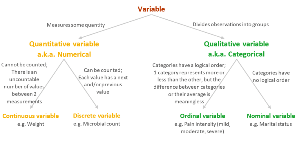
The core difference between them is simple: one is about counting, and the other is about measuring. Let's explore each one.
Discrete Variables: The Countables
A discrete variable is one that can only take on specific, separate values. There are "gaps" between the possible values. Think of these as things you can count in whole numbers.
The video below offers an excellent, straightforward explanation of this concept.
Introduction | Fundamentals of Biostatistics
This clip from "The Statistics Teacher" channel provides a clear definition of discrete variables and why they have distinct "gaps" between values.
Please watch the section explaining discrete random variables. Pay close attention to the hospital admissions example—it perfectly illustrates why you can't have fractional values.
As the video explained, you can have 10, 11, or 12 patient admissions, but you cannot have 10.5 admissions. The values are distinct and countable.
The ACCP's "Biostatistics: A Refresher" workbook also provides a concise definition.
[PDF] Biostatistics: A Refresher - ACCP
This document gives a formal definition of discrete variables in a clinical context.
In the section "II. TYPES OF VARIABLES AND DATA", read the definitions under the heading Discrete Variables. Notice how it categorizes them and provides relevant examples.
Here are some common examples of discrete variables you'll encounter in a pharmacy setting:
- The number of tablets in a prescription.
- The number of adverse events reported during a clinical trial.
- The number of patients in a study group.
- The number of times a patient reports taking their medication correctly in a week.
In all these cases, the variable can only be a whole number (0, 1, 2, 3, etc.).
Continuous Variables: The Measurables
A continuous variable, on the other hand, can take on any value within a given range. There are no gaps; between any two possible values, there is always another possible value. Think of these as things you measure.
Let's return to "The Statistics Teacher" video for the corresponding explanation.
Introduction | Fundamentals of Biostatistics
This segment explains continuous variables, which contrast with the discrete variables we just discussed.
Now, watch the section on continuous random variables. The key idea here is the absence of interruptions or gaps.
The video gives examples like height, weight, and blood pressure. You could be 175 cm tall, or 175.1 cm, or 175.11 cm—the precision is limited only by our measurement tool, not by the nature of the variable itself.
For a pharmacy-specific example, let's look at an article from The Pharmaceutical Journal.
A basic introduction to statistics - The Pharmaceutical Journal
This article provides an excellent, clinically relevant example of a continuous variable within a case study.
Read the section under Types of variables. Focus on the definition of continuous data and the example of LDL cholesterol change from the statin study.
Common examples of continuous variables in pharmacy and health include:
- Blood pressure (e.g., 120.5 mmHg)
- Patient's weight (e.g., 70.2 kg)
- Plasma concentration of a drug (e.g., 15.8 ng/mL)
- Body temperature (e.g., 37.2°C)
Visualizing the Difference
The distinction between discrete and continuous variables becomes very clear when you visualize them. Discrete data is often shown with bar charts, where each bar is separate, representing the "gaps" between values. Continuous data is often represented by a smooth line or curve, showing that any value along that line is possible.

Let's Practice
To solidify your understanding, classify each of the following measurements from a clinical study as either discrete or continuous.
- The number of capsules in a bottle of medication.
- The exact time (in minutes) it takes for a new analgesic to relieve a patient's headache.
- A patient's heart rate in beats per minute (BPM).
- The volume of liquid (in mL) in a cough syrup bottle.
- The number of previous heart attacks a patient has had.
Take a moment to decide on your answers before reading the solutions below.
Solutions:
- Discrete: You can count the capsules. You can't have 29.5 capsules.
- Continuous: Time is measured, not counted. It could be 15 minutes, 15.2 minutes, or 15.21 minutes.
- Discrete: Although heart rate can seem continuous, it is technically a count of beats over a minute. You cannot have 72.5 beats. It is always a whole number. This is a classic tricky example!
- Continuous: Volume is measured and can take any value within a range (e.g., 149.8 mL).
- Discrete: This is a count of events. A patient can have 0, 1, 2, etc., heart attacks, but not 1.5.
Conclusion
This lesson completes our introduction to the fundamental types of data in biostatistics. Understanding these classifications is not just an academic exercise; it's a practical necessity that guides every step of data analysis.
Key Takeaways:
- Quantitative (numerical) variables can be either discrete or continuous.
- Discrete variables are countable and have gaps between values (e.g., number of pills, number of side effects).
- Continuous variables are measurable and can take any value within a range (e.g., blood pressure, weight, drug concentration).
With this foundational knowledge of data types, you are now ready to start working with data. In the next module, we will move on to our first topic in descriptive statistics: organizing raw data by constructing frequency distribution tables. You will see right away how the methods we use to group data depend on whether the data is discrete or continuous.