Hello! Welcome to our next lesson.
In our last session, we discovered that the Discrete Fourier Transform (DFT) has some inherent limitations. By analyzing a finite block of data, we are implicitly using a rectangular window. This leads to spectral leakage, where energy from one frequency "leaks" into others, and the picket-fence effect, where we might mis-measure the true amplitude of a signal. The rectangular window gives excellent frequency resolution but suffers from the worst spectral leakage.
This lesson is all about finding a solution. If the rectangular window is the problem, the solution is to use a different window. We will explore how alternative window functions can dramatically reduce spectral leakage, and we'll analyze the fundamental trade-offs involved.
Your learning outcome for this lesson is to: Apply various window functions (e.g., Hamming, Hanning) to reduce spectral leakage and analyze their trade-offs.
1. The Strategy: Tapering the Signal
The abrupt start and end of our data segment, as defined by the rectangular window, creates sharp discontinuities in the DFT's assumed periodic signal. As you know from your study of Fourier series, discontinuities require a large number of high-frequency components to be represented, which manifests as high side lobes in the frequency domain.
The strategy of windowing is to replace the rectangular window with a function that is shaped to smoothly taper the signal's amplitude to zero at both ends of the segment. This reduces the severity of the discontinuity, which in turn reduces the energy in the side lobes of the window's spectrum.
To start, let's watch a brief conceptual overview. This video clearly illustrates why we need windows and how they work at a high level.
Please watch the first two sections of the 'Window Functions' video: 0:00 - 1:58: This will be a quick recap of how the discontinuity caused by finite sampling leads to spectral leakage. 1:58 - 3:36: This part introduces the core idea of windowing: multiplying the time signal by a tapering function, which corresponds to convolving their spectra.
The key takeaway is this: applying a window is a multiplication in the time domain. By the convolution theorem, this means the resulting spectrum is the convolution of the signal's true spectrum with the Fourier transform of the window function. Our goal is to choose a window function whose transform has much lower side lobes than the sinc function of the rectangular window.
2. The Raised-Cosine Family: Hanning and Hamming Windows
Among the most common and historically significant window functions are the Hanning and Hamming windows. They belong to a family of "raised-cosine" windows.
The Hanning Window
Named after the Austrian meteorologist Julius von Hann, the Hanning window (often misspelled "Hanning") is a simple, effective window defined by a raised cosine curve. It smoothly tapers to zero at its endpoints.
For a DFT of length , the Hanning window sequence for is defined as:
The genius of this construction lies in the frequency domain. The Fourier transform of this window can be derived as the sum of three shifted Dirichlet kernels (the transform of a rectangular window). These kernels are arranged in such a way that their side lobes are in phase opposition and partially cancel each other out, leading to much lower overall side lobe levels compared to the rectangular window alone.
The Hamming Window
Proposed by the renowned mathematician Richard Hamming, this window is a subtle but clever modification of the Hanning window. Its definition is very similar:
Notice the coefficients (0.54 and 0.46). Unlike the Hanning window, the Hamming window does not go all the way to zero at its endpoints. This small discontinuity is intentional. The coefficients are specifically chosen to place a zero in the window's frequency response that precisely cancels the largest, first side lobe. This results in even better suppression of the nearest side lobes, but at the cost of a slower overall decay rate for side lobes further away.
The Wikipedia article on 'Window function' provides clear, standardized definitions for these windows.
Please read the short subsections on the Hann window and the Hamming window. Focus on their mathematical definitions and the brief explanation of why the Hamming window's coefficients are chosen.
3. Quantifying the Trade-off: Figures of Merit
We've established a fundamental trade-off: reducing side lobe level (leakage) seems to come at the cost of widening the main lobe (resolution). To make an informed choice for a given application, we need a more rigorous way to compare windows.
For this, we turn to a classic and highly influential paper in the field by F.J. Harris. It provides the deep mathematical treatment you appreciate and establishes the standard metrics for evaluating window performance.
Windows, Harmonic Analysis and the Discrete Fourier Transform
The paper 'Windows, Harmonic Analysis and the Discrete Fourier Transform' is a foundational text on this topic. We will focus on the section that defines the key performance metrics.
Please read Section III. WINDOWS AND FIGURES OF MERIT (pages 9-18). This is the most critical part of the lesson. As you read, focus on understanding the definitions and significance of these key parameters: Equivalent Noise Bandwidth (ENBW): How much broadband noise the window's spectrum will pass. Scalloping Loss: The maximum signal loss due to the picket-fence effect. Spectral Leakage: Described by the peak sidelobe level and the sidelobe roll-off rate. This is the most important metric for finding weak signals near strong ones. Minimum Resolution Bandwidth: The ability to distinguish two closely spaced sinusoids. Harris argues for using the 6-dB bandwidth for this metric.
Now, let's use the information from that paper, specifically Table I on page 19, to compare the windows we've discussed:
| Window | Main Lobe Width (-3 dB bins) | Peak Sidelobe Level (dB) | Sidelobe Roll-off (dB/oct) |
|---|---|---|---|
| Rectangle | 0.89 | -13.3 | -6 |
| Hanning | 1.44 | -31.5 | -18 |
| Hamming | 1.30 | -42.7 | -6 |
This table quantifies the trade-offs perfectly:
- Hanning vs. Rectangle: The Hanning window widens the main lobe by about 60% (
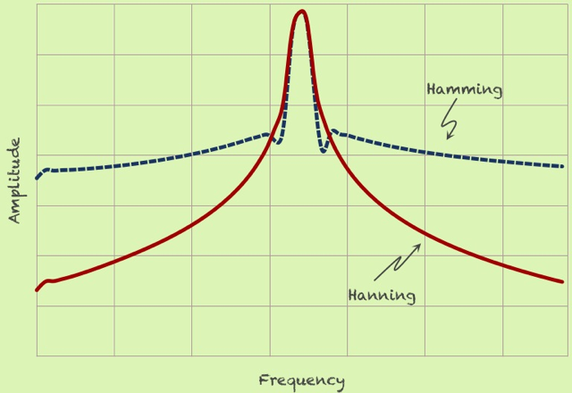
1.44/0.89), degrading resolution. However, its peak side lobe is -31.5 dB, a huge improvement over the rectangular window's -13.3 dB. It also has a much faster side lobe roll-off rate (-18 vs -6 dB/octave). - Hamming vs. Hanning: The Hamming window has a narrower main lobe than Hanning, offering slightly better resolution. Its key feature is the extremely low peak side lobe (-42.7 dB), making it excellent for rejecting leakage from adjacent frequencies. However, its side lobes roll off very slowly (-6 dB/octave), meaning leakage from frequencies far away can be higher than with the Hanning window.
Let's visualize this comparison.
4. A Practical Demonstration: Resolving a Weak Tone
Theory and tables are essential, but seeing the effect in action provides true insight. The Harris paper includes a powerful experiment: trying to detect a weak sine wave in the presence of a strong one that is only a few DFT bins away.
The signal consists of two tones:
- A strong tone at frequency .
- A weak tone, 40 dB quieter, at frequency .
Let's see what happens when we analyze this signal using different windows.
1. Rectangular Window (Figure 51 in the Harris paper): The strong tone is at 10.5 bins. Its spectral leakage, from the -13 dB side lobes, completely swamps the weak tone at bin 16. The weak tone is invisible.
2. Hanning Window (Figure 55): A massive improvement! The leakage from the strong tone is suppressed enough that we can clearly see the peak of the weak tone. The lower side lobes have "uncovered" it.
3. Hamming Window (Figure 58): Similar to the Hanning, the weak tone is clearly detected. Thanks to the Hamming window's even lower first side lobe, the "floor" of the noise created by leakage is lower, making the detection even more robust.
This experiment vividly demonstrates the power of windowing. Without it, measuring signals with a large dynamic range would be nearly impossible.
Test your understanding!
You are tasked with two different spectral analysis problems:
Problem A: You need to measure the precise frequency of two tones that you know are very close together and have roughly equal amplitude.
Problem B: You need to detect a very faint, high-frequency harmonic in the presence of a very strong fundamental tone. The harmonic is relatively far in frequency from the fundamental.
For each problem, which performance metric is most critical: main lobe width, peak sidelobe level, or sidelobe roll-off rate? Based on that, which of the three windows (Rectangular, Hanning, Hamming) would you choose, and why?
Show answer
Problem A:
- Critical Metric: Main lobe width. To distinguish two closely spaced tones (i.e., for high resolution), you need the narrowest possible main lobe.
- Window Choice: Rectangular. Since the tones are of equal amplitude, spectral leakage from one is unlikely to obscure the other. The rectangular window offers the narrowest main lobe and thus the best ability to resolve the two distinct peaks.
Problem B:
- Critical Metric: Sidelobe roll-off rate. The strong fundamental tone's leakage will be the primary source of interference. Since the faint harmonic is far away, we care most about how much the leakage is attenuated at greater frequency distances.
- Window Choice: Hanning. The Hanning window's side lobes roll off at -18 dB/octave, much faster than the Hamming or Rectangular window's -6 dB/octave. This means it will provide better suppression of leakage far from the main lobe, giving you the best chance to see the faint, distant harmonic. The Hamming window, while having a very low first side lobe, has higher side lobes further out, which could obscure the signal of interest in this case.
Conclusion
In this lesson, we've moved from identifying the problem of spectral leakage to actively solving it with window functions. You've seen that there's no single "best" window, only the "right" window for a given task.
Key Takeaways:
- Window functions reduce spectral leakage by tapering the signal to zero at its boundaries, lessening the discontinuity seen by the DFT.
- The primary trade-off in window selection is between frequency resolution (governed by main lobe width) and spectral leakage (governed by side lobe height and roll-off rate).
- The Hanning window offers a good general-purpose balance, significantly reducing leakage with a modest loss of resolution. Its side lobes decay quickly.
- The Hamming window is optimized to minimize the highest side lobe, making it excellent for rejecting leakage from very close, strong signals. However, its far-out side lobes are higher than the Hanning's.
- The choice of window is application-dependent, based on whether you need to resolve closely-spaced components or detect weak components in the presence of strong ones.
Preview of the Next Lesson:
We've seen that applying a window (multiplication in time) results in a convolution in the frequency domain. In the next lesson, we will investigate the specific type of convolution implied by the DFT's multiplication property. We will derive the concept of circular convolution from the DFT multiplication property and distinguish it from the linear convolution we've been discussing in the context of the DTFT. This is a crucial and often misunderstood property of the DFT.