Deriving the DFT from DTFT Sampling

Hello! Welcome to your next lesson.

In our last session, we traveled through history to understand the significance of the Fast Fourier Transform (FFT). We saw that the challenge of analyzing large datasets, like seismic signals during the Cold War, made the $O (N^{2})$ complexity of a direct DFT calculation prohibitively slow. The "re-discovery" of the FFT by Cooley and Tukey in 1965, with its efficient $O (N lo g N)$ complexity, was the watershed moment that launched the modern era of digital signal processing.

Now that we appreciate why we need an efficient algorithm, it's time to formally define the transform it calculates. Our previous work with the z-transform and the Discrete-Time Fourier Transform (DTFT) provided the theoretical foundation for frequency analysis of discrete signals. However, the DTFT produces a spectrum that is a continuous function of frequency, which is impossible to compute or store on a digital machine.

Today, we will bridge this gap between theory and practice. Our learning outcome is to derive the Discrete Fourier Transform (DFT) by sampling the DTFT spectrum. We will see how this sampling process transforms the continuous DTFT into a finite, computable set of frequency components, establishing the DFT as the cornerstone of practical frequency analysis in DSP.

1. The Need for a Discrete Spectrum

Let's begin with a discrete-time signal, $x [n]$ , that is non-zero only for a finite duration, say $n = 0, 1, \dots, N - 1$ . In a previous module, we defined its Discrete-Time Fourier Transform (DTFT) as:

X (e^{j ω}) = n = - \infty \sum \infty x [n] e^{- j ω n}

Since our signal is of finite duration, this simplifies to:

X (e^{j ω}) = n = 0 \sum N - 1 x [n] e^{- j ω n}

While this sum is finite and seems computable, there's a problem: the frequency variable $ω$ is continuous. To represent $X (e^{j ω})$ fully, we would need to calculate its value at an infinite number of frequencies. This is not practical for any digital computer.

The logical next step, which is central to all digital signal processing, is to sample the continuous frequency spectrum.

2. Deriving the DFT by Sampling the DTFT

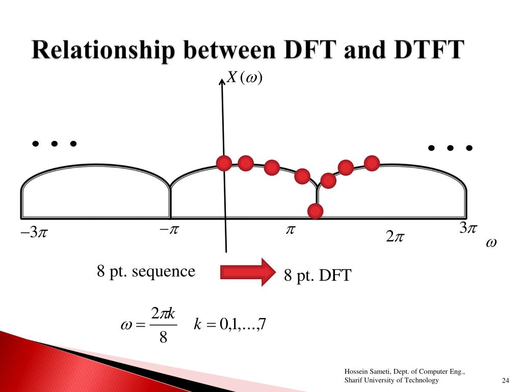
If we are to sample the DTFT, we need to choose our sample points. A natural and mathematically convenient choice is to take $N$ uniformly spaced samples over one full period of the DTFT, which is $2 π$ . This means we will evaluate the DTFT at the following discrete frequencies:

ω_{k} = \frac{2 π}{N} k for k = 0, 1, \dots, N - 1

By substituting these discrete frequencies $ω_{k}$ into the DTFT equation, we arrive at the definition of the N-point Discrete Fourier Transform (DFT).

The Discrete Fourier Transform: Sampling the DTFT

The following video from Barry Van Veen provides a clear and concise derivation of the DFT. It walks through the exact logic we just discussed: starting with the DTFT of a finite-duration signal and then sampling the frequency variable \omega.

Please watch from 1:35 to 4:14. Pay close attention to how the continuous variable \omega in the DTFT is replaced by the discrete frequency points \omega_k to yield the DFT equation.

As the video explains, the DFT, denoted as $X [k]$ , is simply the DTFT $X (e^{j ω})$ evaluated at these $N$ frequency points:

X [k] ≜ X (e^{j ω_{k}}) = n = 0 \sum N - 1 x [n] e^{- j (\frac{2 π}{N} k) n} for k = 0, 1, \dots, N - 1

This is the analysis equation for the N-point DFT. It takes an N-point time-domain sequence $x [n]$ and transforms it into an N-point frequency-domain sequence $X [k]$ . Crucially, every part of this formula is discrete and finite, making it perfectly suited for a computer.

The following image provides an excellent visual summary of this relationship.

Relationship between DFT and DTFT through Sampling — The DFT (red dots) consists of N samples of the continuous DTFT spectrum (blue curve). The samples are taken at uniform frequency intervals of $\Delta\omega = 2\pi/N$ over one period of the DTFT.

3. A Worked Example

To make this derivation concrete, let's see how it works for a simple signal. Consider a 4-point rectangular pulse:

x [n] = {1, 1, 1, 1} for n = 0, 1, 2, 3

Here, $N = 4$ . The DFT will give us 4 frequency samples, $X [0], X [1], X [2], X [3]$ .

The Discrete Fourier Transform: Sampling the DTFT

Let's return to the same video, which now provides a step-by-step example using this exact 4-point pulse. It first calculates the DFT directly and then shows that the result matches the values of the signal's DTFT at the sampling points \omega_k = rac{2\pi}{4}k = rac{\pi}{2}k.

Watch from 4:14 to 8:06. This section will help solidify the connection between the DFT and DTFT by demonstrating their equivalence at the sampling frequencies.

As the example showed, the 4-point DFT of $x [n] = {1, 1, 1, 1}$ is $X [k] = {4, 0, 0, 0}$ . This result is obtained by evaluating the DTFT of the pulse, which has a sinc-like shape, at the frequencies $ω_{0} = 0$ , $ω_{1} = π /2$ , $ω_{2} = π$ , and $ω_{3} = 3 π /2$ . The DTFT happens to have its peak at $ω = 0$ and zero-crossings at the other sample points for this specific signal and choice of $N$ .

Test your understanding!

Suppose you have a 3-point signal $x[n] = \{1, 2, 1\}$. You want to compute its 3-point DFT.

What are the discrete frequencies $ω_{k}$ at which you are sampling the DTFT?
Write out the expression for $X [1]$ , the DFT component corresponding to $k = 1$ . You don't need to compute the final numeric value.

Show answer

For an $N = 3$ point DFT, the sampling frequencies are:
- $ω_{0} = \frac{2 π}{3} \cdot 0 = 0$
- $ω_{1} = \frac{2 π}{3} \cdot 1 = \frac{2 π}{3}$
- $ω_{2} = \frac{2 π}{3} \cdot 2 = \frac{4 π}{3}$
The general DFT formula is $X [k] = \sum_{n = 0}^{N - 1} x [n] e^{- j \frac{2 π}{N} k n}$ .
For $N = 3$ and $k = 1$ , this becomes:
$X [1] = n = 0 \sum 2 x [n] e^{- j \frac{2 π}{3} (1) n} = x [0] e^{0} + x [1] e^{- j \frac{2 π}{3}} + x [2] e^{- j \frac{4 π}{3}}$
Substituting the values of $x [n]$ :
$X [1] = 1 \cdot e^{0} + 2 \cdot e^{- j \frac{2 π}{3}} + 1 \cdot e^{- j \frac{4 π}{3}}$

4. Duality: The Consequence of Sampling in Frequency

Your background in signal processing has introduced you to the concept of duality in Fourier analysis. For instance, a time shift in a signal corresponds to a phase shift in its frequency spectrum, while a frequency shift (modulation) corresponds to a phase shift in the time domain.

This duality also applies to sampling. In the "Sampling and Reconstruction" module, we will formally derive that sampling a signal in the time domain causes its spectrum to become periodic in the frequency domain. The dual of this is also true: sampling a spectrum in the frequency domain (which is what we did to get the DFT) causes the signal to become periodic in the time domain.

This phenomenon is sometimes called time-domain aliasing.

Chapter 4 - THE DISCRETE FOURIER TRANSFORM

For a more formal treatment of this concept, let's turn to a chapter from a set of lecture notes from MIT. It provides a mathematically rigorous explanation of what happens in the time domain when we sample in the frequency domain.

Please read section 4.1.2, titled 'Condition for signal reconstruction from the DFT'. Focus on understanding Equation (4.3), which shows that the inverse transform of the sampled spectrum is a periodic sum of shifted copies of the original signal. This is the mathematical basis for time-domain aliasing.

As the text explains, sampling the spectrum $X (e^{j ω})$ at intervals of $1/ N$ (in normalized frequency, equivalent to $2 π / N$ in radians) results in an inverse transform $x ~ [n]$ that is a periodic repetition of the original signal $x [n]$ :

x ~ [n] = r = - \infty \sum \infty x [n - r N]

(Note: The resource includes a scaling factor of N, which we can disregard for this conceptual point).

This has a critical implication: If our original signal $x [n]$ has a duration that is longer than $N$ , the repeated copies will overlap and corrupt each other. However, in our standard use case, we define the DFT length $N$ to be equal to the signal's duration. In this case, $x [n]$ is zero for $n \geq N$ , so the periodic copies don't overlap, and no information is lost. This allows us to perfectly reconstruct the original signal from its DFT.

5. The Inverse DFT

The fact that an $N$ -point signal can be losslessly represented by its $N$ -point DFT means there must be an inverse transform. The Inverse Discrete Fourier Transform (IDFT) reconstructs the time-domain signal $x [n]$ from its frequency components $X [k]$ .

Chapter 4 - THE DISCRETE FOURIER TRANSFORM

Let's look at the next section of the same MIT notes, which derives this inverse relationship.

Please read section 4.1.3, 'Inverse discrete Fourier transform'. You can skim the two proofs, but focus on the final result: the DFT pair given by equations (4.5a) and (4.5b).

The DFT pair for a finite-duration signal is:

Analysis (DFT):

X [k] = n = 0 \sum N - 1 x [n] e^{- j \frac{2 π}{N} k n}

Synthesis (IDFT):

x [n] = \frac{1}{N} k = 0 \sum N - 1 X [k] e^{j \frac{2 π}{N} k n}

Observe the beautiful symmetry between the two equations. They are nearly identical, differing only in the sign of the exponent and the $1/ N$ scaling factor in the inverse. The synthesis equation tells us that any finite-duration signal $x [n]$ can be represented as a sum of $N$ discrete complex sinusoids whose frequencies are $f_{k} = k / N$ (normalized) and whose complex amplitudes are given by the DFT coefficients $X [k]$ .

Conclusion

In this lesson, we made the pivotal transition from the continuous world of the DTFT to the discrete, computable world of the DFT. We established that the DFT is not a new or different transform, but rather a specific, sampled representation of the DTFT.

Key Takeaways:

The DFT is derived by taking $N$ uniform samples of the DTFT over the frequency interval $[0, 2 π)$ .
The frequency samples are located at $ω_{k} = \frac{2 π}{N} k$ .
This sampling in the frequency domain implies a periodic extension of the signal in the time domain (time-domain aliasing).
For a signal of duration $N$ , an $N$ -point DFT contains all the signal's information, and the original signal can be perfectly recovered using the IDFT.
The DFT analysis and IDFT synthesis equations form a transform pair that is the foundation of computational frequency analysis.

Preview of the Next Lesson:

We have now established the relationship between the DFT and the DTFT. In our next lesson, we will complete the picture by connecting these concepts to the z-transform. The learning outcome is to analyze the relationship between the DFT, DTFT, and z-transform, interpreting the DFT as samples of the z-transform on the unit circle. This will unify the different discrete-time analysis tools we have studied and provide an even deeper insight into what the DFT represents.

Recommended resources