Delay-Based Audio Effects

1. The Digital Delay Line

The heart of any delay-based effect is the delay line. In the digital domain, this is simply a segment of memory used to store a stream of audio samples. As new samples come in, they are written to the buffer, and the output of the delay line is read from an earlier position in that same buffer. To manage memory efficiently, this is almost always implemented as a circular buffer (or ring buffer).

The following video provides an excellent explanation of the delay line and its core parameters.

As the video explains, the crucial relationship is:
$D\text{ (samples)}=T_d\text{ (seconds)}\times f_s\text{ (samples/second)}$
This simple equation is the foundation for setting the timing of all delay-based effects. The size of this buffer is a key practical consideration, as longer delay times at high sample rates can require significant amounts of RAM.

2. From Delay to Echo

The simplest delay effect is a single, discrete echo, often called "slap-back." We create this by mixing the original "dry" signal with a delayed version of it.

This can be described by the following difference equation:
$y[n]=x[n]+\alpha \cdot x[n-D]$
where:

• $x[n]$ is the input signal.
• $y[n]$ is the output signal.
• $D$ is the delay length in samples.
• $\alpha$ is the "mix" or "depth" of the echo, where $0<\alpha \le 1$.

You'll recognize this as a simple two-tap Finite Impulse Response (FIR) filter. Its impulse response is just two impulses: one at $n=0$ and another at $n=D$. In the z-domain, its transfer function is:
$H(z)=\frac{Y(z)}{X(z)}=1+\alpha z^{-D}$
This is also known as a feed-forward comb filter, which creates a series of uniformly spaced notches in the frequency spectrum.

3. Creating Endless Echoes with Feedback

While a single echo is useful, most iconic delay effects feature a series of echoes that gradually fade away. We can achieve this efficiently by adding feedback—taking the output of the delay line, scaling it, and adding it back to the input. This creates an Infinite Impulse Response (IIR) structure.

Let's watch a clear explanation of this fundamental feedback delay architecture.

Mathematical Analysis

Let's analyze the core feedback loop shown in the video, assuming for a moment that the output is taken directly after the delay line (a "fully wet" signal). The signal being fed into the delay line, $w[n]$, is the sum of the input signal $x[n]$ and the scaled, delayed output $G\cdot y[n]$. The output $y[n]$ is simply the input to the delay line, delayed by $D$ samples.

This gives us:
$y[n]=w[n-D]=x[n-D]+G\cdot y[n-D]$

This is a first-order recursive equation, defining an IIR filter. To find the transfer function, we take the z-transform:
$Y(z)=z^{-D}X(z)+G{z}^{-D}Y(z)$
$Y(z)(1-G{z}^{-D})=z^{-D}X(z)$
$H(z)=\frac{Y(z)}{X(z)}=\frac{z^{-D}}{1-G{z}^{-D}}$

This is the transfer function of a classic feedback comb filter.

Stability Analysis

As with any IIR filter, we must ensure stability. The poles of the system are the roots of the denominator of $H(z)$.
$1-G{z}^{-D}=0⟹z^D=G$
This equation has $D$ roots (the poles) distributed on a circle of radius $|G{|}^{1/D}$ in the z-plane. For the system to be stable, all poles must lie inside the unit circle. This requires:
$|G{|}^{1/D}<1⟹|G|<1$
This confirms our intuition: if the feedback gain $|G|$ is 1 or greater, the echoes will never decay and will instead remain constant or grow exponentially, leading to instability.

4. The Architecture of Reverberation

Reverberation can be thought of as an extremely dense collection of echoes. When a sound is made in a real room, the sound waves reflect off every surface, creating thousands of reflections that arrive at the listener's ears at different times and from different directions.

Simulating every single reflection is computationally prohibitive. Therefore, algorithmic reverberation does not attempt to model the physics perfectly. Instead, it uses a network of delay lines to create a psychoacoustically convincing impression of a reverberant space.

The Schroeder Reverberator

The pioneering work in this area was done by Manfred Schroeder in the 1960s. He proposed combining two types of simple delay-based filters:

1. Comb Filters: Several parallel feedback comb filters (like the one we just analyzed) with different, mutually prime delay lengths. These create the initial echo density that simulates early reflections.
2. All-Pass Filters: The output of the comb filters is then fed through a few all-pass filters in series. An all-pass filter has a flat magnitude response but a non-linear phase response. Its purpose is not to change the tone, but to "smear" the signal in time, increasing the echo density and making the sound smoother and more diffuse, less like a series of distinct echoes.

The transfer function of a simple all-pass filter is:
$H_{AP}(z)=\frac{-g+z^{-D}}{1-g{z}^{-D}}$
Notice how the zero at $z^D=1/g$ is at the reciprocal location of the pole at $z^D=g$, which is what gives it an all-pass characteristic.

Modern reverbs often use more complex structures like Feedback Delay Networks (FDN), which use a matrix to mix and feed the outputs of multiple delay lines back to their inputs, allowing for a very rich and complex response.

5. Reverberation Time (T60)

A key parameter of any reverb effect is the reverberation time, or T60. This is defined as the time it takes for the impulse response's energy to decay by 60 decibels (dB). In our simple feedback comb filter, the T60 is directly controlled by the feedback gain $G$ and the delay length $D$.

With each pass through the delay loop of length $D$, the amplitude is multiplied by $G$. The amplitude decay in dB per second is:
$\text{Decay (dB/sec)}=\frac{20{\log }_{10}(|G|)}{T_d}=\frac{20{\log }_{10}(|G|)}{D/f_s}$
To find the time to decay by 60 dB, we set:
$T_{60}=\frac{-60}{\text{Decay (dB/sec)}}=T_d\cdot \frac{-60}{20{\log }_{10}(|G|)}=T_d\cdot \frac{-3}{{\log }_{10}(|G|)}$
This formula directly links the filter parameters to the perceptual result.

Test your understanding!

The problem below describes a single feedback loop. Using the relationship between feedback gain and reverberation time, calculate the T60 for this system.

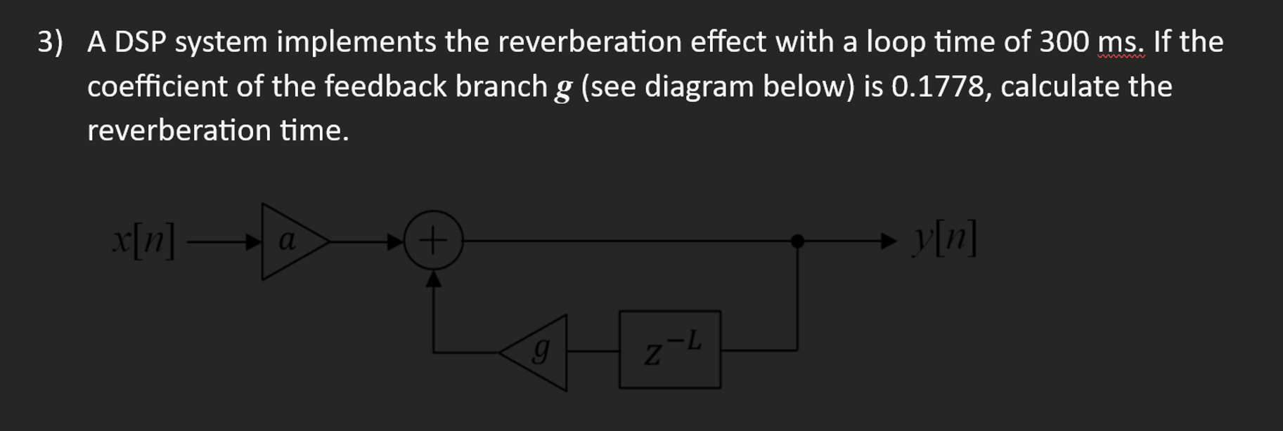
Show answer

We can calculate the decay in dB for one pass through the loop:
$\text{Decay per loop (dB)}=20{\log }_{10}(g)=20{\log }_{10}(0.1778)\approx 20\cdot (-0.75)=-15\text{ dB}$
The number of loops required for a 60 dB decay is:
$\text{Number of loops}=\frac{-60\text{ dB}}{-15\text{ dB/loop}}=4\text{ loops}$
Since each loop takes 300 ms, the total reverberation time is:
$T_{60}=4\text{ loops}\times 300\text{ ms/loop}=1200\text{ ms}=1.2\text{ seconds}$

6. Implementation in Practice

We now have all the theoretical components. Let's see how they are assembled in a practical software implementation. The LINK video walks through a C-code implementation of the feedback delay effect we've analyzed.

The code directly translates the block diagram into a step-by-step process: read from the delay line, compute the new value to write, write it, update the pointers, and compute the final mixed output.

Conclusion

In this lesson, we explored the world of delay-based audio effects, connecting simple DSP principles to classic sounds used in music production for decades.

Key Takeaways:

• The core of delay effects is the delay line, a circular buffer that stores and retrieves past audio samples.
• A simple echo is an FIR filter (feed-forward comb filter) that adds a delayed signal to the original.
• Creating decaying echoes requires an IIR filter (feedback comb filter), whose stability depends on the feedback gain $|G|<1$. The transfer function is $H(z)=z^{-D}/(1-G{z}^{-D})$.
• Reverberation is a complex sonic texture created by simulating thousands of echoes. Algorithmic reverbs use networks of comb and all-pass filters (e.g., Schroeder, FDN) to create a psychoacoustically realistic effect.
• The reverberation time (T60) is determined by the interplay of delay length and feedback gain.

Preview of the Next Lesson:

We have now manipulated signals in both the frequency domain (EQ) and the time domain (delay/reverb). In our next lesson, "Analyze and implement dynamic range compression and limiting," we will shift our focus to the amplitude domain. We will learn how to build processors that automatically control the volume of a signal, a fundamental technique in audio engineering.