Spectral Analysis with Windowing and STFT

1. The Problem: Signals that Change

The Discrete Fourier Transform (DFT), which you've studied extensively, operates on a finite block of data. It implicitly assumes that this block represents one period of an infinitely repeating signal.

This assumption holds for stationary signals (like a pure sine wave), but it breaks down for real-world audio. When you grab a random chunk of a song or speech, the signal at the end of the chunk doesn't smoothly connect back to the beginning.

The solution is not to analyze the entire signal at once, but to break it into short, overlapping segments. The idea is that over a very short duration (e.g., 20-40 milliseconds), a complex audio signal can be considered "quasi-stationary"—its frequency content doesn't change too much.

By performing a DFT on each of these short segments, we can build a picture of how the spectrum evolves over time. This is the fundamental concept behind the Short-Time Fourier Transform.

2. Windowing: Taming the Discontinuities

Simply chopping the signal into segments, or frames, still creates artificial discontinuities at the edges. To mitigate the resulting spectral leakage, we multiply each frame by a window function. A window function is a finite-length sequence that is zero at its ends and typically smooth and bell-shaped in the middle.

Multiplying our signal frame by a window function tapers its values gracefully to zero at the boundaries. This ensures that when the DFT assumes the frame is periodic, the sharp discontinuities are gone.

To get a clear visual intuition of this entire process—framing, windowing, and the introduction of an overlap or hop size—let's watch a segment of the following video.

This process of sliding a window along the signal, taking the DFT of each windowed frame, and stacking the results is the essence of the STFT.

3. The Short-Time Fourier Transform (STFT)

Now, let's formalize this process. Your background in signal processing will be very useful here, as the STFT is a direct and logical extension of the DFT.

As the video explains, the STFT, $X[n,k]$, is a two-dimensional function of time (frame index $n$) and frequency (bin index $k$). The equation is:

where:

• $x[m]$ is the input signal.
• $w[m]$ is the window function.
• $n$ is the time index, representing the position of the window.
• $k$ is the frequency index.
• $N$ is the size of the DFT.

This equation looks complex, but it describes exactly what we've been discussing: for each time step $n$, it computes the DFT of the signal $x[m]$ as seen through the shifted window $w[n-m]$.

The spectrogram, which we use for visualization, is simply the squared magnitude of the STFT:

Since we are now dealing with real-valued magnitudes, we can plot this as an image, with time on one axis, frequency on the other, and intensity/color representing the energy at that time-frequency point.

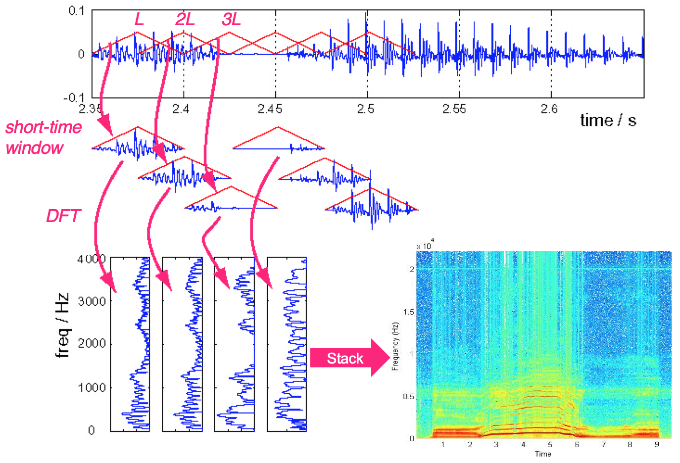
4. The Time-Frequency Resolution Trade-off

The choice of the window function's length is the most critical parameter in STFT analysis. It forces a fundamental trade-off, which has its roots in the uncertainty principle you may have encountered in Fourier analysis or quantum mechanics.

• A long window provides good frequency resolution. Because the window covers a longer time duration, the DFT can better distinguish between closely spaced frequency components. However, any rapid changes within that long window will be averaged out, leading to poor time resolution.
• A short window provides good time resolution. It can pinpoint transient events in the signal very accurately. However, the short observation time makes it difficult to resolve fine frequency details, leading to poor frequency resolution.

Let's see a practical demonstration of this trade-off.

This trade-off is unavoidable. The choice of window length depends entirely on the application. For analyzing the pitch of musical notes, a longer window is often better to resolve harmonics. For detecting a drum hit or a speech plosive, a shorter window is preferred.

5. Alternative Interpretations of the STFT

Given your background in electrical engineering, you will appreciate that the STFT can be interpreted in ways other than a sequence of DFTs. These alternative views are mathematically equivalent but offer different insights.

The filter bank interpretation is particularly powerful and common in signal processing. It recasts the STFT as a bank of equally spaced, identical bandpass filters. The bandwidth of each filter is determined by the Fourier transform of the window function. This neatly explains the time-frequency trade-off: a narrow-bandwidth filter (good frequency resolution) requires a long impulse response (poor time resolution), and vice versa.

Conclusion

Today, we've developed the essential tool for practical audio analysis. We moved from the static, time-averaged view of the DFT to the dynamic, time-varying representation of the STFT and the spectrogram.

Key Takeaways:

• Real-world audio signals are non-stationary, and analyzing them with a single DFT leads to spectral leakage.
• The STFT overcomes this by analyzing a sequence of short, overlapping, windowed frames of the signal.
• Window functions (e.g., Hann, Hamming) taper the frames to zero at the edges to reduce artificial discontinuities.
• The spectrogram, or the squared magnitude of the STFT, is a time-frequency representation that allows us to visualize how a signal's spectrum evolves.
• There is a fundamental time-frequency resolution trade-off controlled by the window length: long windows give good frequency resolution, while short windows give good time resolution.
• The STFT can also be interpreted as a filter bank, which provides a powerful link to your knowledge of LTI systems.

Preview of the Next Lesson:

Now that we have the tools to analyze the frequency content of audio over time, the next logical step is to modify it. In our next lesson, we will begin our study of digital filters, focusing on how to design and apply digital filters for audio equalization and tone control. We will use our understanding of the spectrogram to design filters that can boost, cut, or isolate specific frequency bands in an audio signal.