FIR Filter Design: Frequency Sampling Method

1. The Core Idea: From Frequency Samples to Filter Taps

Recall that a filter's impulse response, $h[n]$, and its continuous frequency response, $H(e^{j\omega })$, are related by the Discrete-Time Fourier Transform (DTFT) pair:
$h[n]=\frac{1}{2\pi }{\int }_{-\pi }^{\pi }H(e^{j\omega })e^{j\omega n}d\omega$

For an ideal filter, like a "brick-wall" low-pass filter, $H(e^{j\omega })$ is well-defined. However, as we saw in the last lesson, the resulting $h[n]$ is an infinitely long sinc function. The window method tackled this by truncating $h[n]$.

The frequency sampling method approaches this differently. Instead of solving the integral analytically, we approximate it using a numerical technique you've likely encountered in calculus: a Riemann sum.

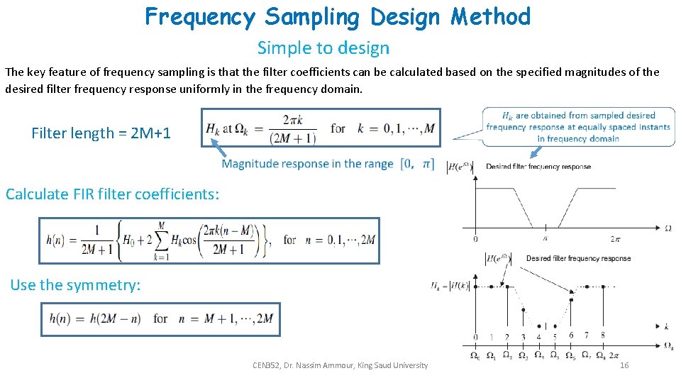
As the resource explains, by sampling the desired frequency response $H_d(e^{j\omega })$ at $N$ equally spaced frequencies ${\omega }_k=\frac{2\pi k}{N}$, we transform the continuous integral into a discrete sum. The resulting approximation for the impulse response $h[n]$ is precisely the N-point IDFT of the frequency samples $H[k]=H_d(e^{j{\omega }_k})$:

$h[n]=\frac{1}{N}{\sum }_{k=0}^{N-1}H[k]e^{j2\pi nk/N},\text{for }n=0,1,\dots ,N-1$

This gives us a simple, powerful, three-step procedure for designing an FIR filter of length $N$:

1. Define the ideal frequency response, $H_d(e^{j\omega })$.
2. Sample $H_d(e^{j\omega })$ at $N$ points to get the discrete frequency samples, $H[k]$.
3. Calculate the N-point IDFT of $H[k]$ to obtain the $N$ filter coefficients, $h[n]$.

2. The Catch: Time-Domain Aliasing

You know from sampling theory that sampling a signal in the time domain causes its spectrum to become periodic in the frequency domain. The duality principle of the Fourier transform implies the reverse: sampling in the frequency domain causes the time-domain signal to become periodic.

When we use the IDFT to find $h[n]$, we are implicitly creating a periodic version of the ideal impulse response. For a typical low-pass filter, the ideal impulse response is a sinc function, which is infinitely long. The frequency sampling process effectively causes this infinite sinc function to be repeated every $N$ samples. The tails of the infinitely repeating sinc functions "wrap around" and add to the main lobe of the primary period. This effect is called time-domain aliasing.

This figure from the Stack Exchange article illustrates time-domain aliasing. The ideal impulse response (a sinc function) is infinite. Sampling in the frequency domain creates a periodic version of this signal, where the tails from adjacent periods overlap, distorting the impulse response within the primary period of N samples.

What's the consequence?
The frequency response of the filter we design will be perfect at the sample points ${\omega }_k$. However, between these sample points, the response can deviate significantly, often resulting in large ripples in the passband and poor attenuation in the stopband. This is the primary drawback of the basic frequency sampling method compared to the windowing method for an equivalent filter length.

3. A Practical Design Procedure

Despite its limitations, the frequency sampling method is straightforward to implement. Let's walk through the practical steps, including an important detail for ensuring the filter coefficients are real.

The video highlights a crucial point. For the impulse response $h[n]$ to be real-valued, its DFT, $H[k]$, must have complex conjugate symmetry: $H[k]=H^{\ast }[N-k]$. The modified IDFT formulas shown in the video are simply efficient ways of computing the IDFT while enforcing this symmetry, saving you from calculating the full complex sum.

Now, let's see this procedure applied to a concrete example.

4. Evaluating the Method and Looking Ahead

So, when is the frequency sampling method useful?

• Pros: It's conceptually straightforward and provides perfect accuracy at the specified frequency sample points. This can be ideal for applications where performance at specific frequencies is critical (e.g., building a filter to reject a specific set of harmonics).

• Cons: For general-purpose selective filters (like low-pass or band-pass), the performance between sample points is often poor due to time-domain aliasing. It typically yields much worse stopband attenuation than a filter designed with the window method using the same number of coefficients.

An important extension to this method involves not making the transition from passband to stopband so abrupt. Instead of samples being strictly 1 or 0, one or two samples in the transition band can be set to values between 0 and 1. By carefully optimizing the values of these transition samples, the stopband ripple can be significantly reduced. This idea of optimizing parameters to minimize error is a key concept that leads to more advanced design techniques.

Conclusion

In this lesson, we explored the frequency sampling method, which offers a distinct alternative to the windowing technique for FIR filter design.

Key Takeaways:

• The frequency sampling method designs a filter by sampling the desired frequency response and then using the IDFT to compute the filter coefficients.
• Mathematically, it can be understood as a Riemann sum approximation of the continuous inverse DTFT integral.
• Its primary limitation is time-domain aliasing, which arises from sampling in the frequency domain and results in poor performance (ripple, low attenuation) between the sample points.
• The method is most effective when the desired response is only critical at specific, uniformly spaced frequencies.

Preview of the Next Lesson:

Both the window and frequency sampling methods are intuitive but are ultimately sub-optimal. They do not produce the best possible filter for a given length and set of specifications. This raises a natural question: Can we design a filter that has the absolute minimum possible error, distributed evenly across the passband and stopband? The answer is yes. This leads us to the concept of "optimal" filters, and in our next lesson, we will describe the principles of the celebrated Parks-McClellan algorithm, which is used to design such optimal equiripple FIR filters.