Chebyshev Filter Approximations and Equiripple Analysis

1. The Key Ingredient: Chebyshev Polynomials

Before we can even talk about the filters, we must understand their mathematical foundation: the Chebyshev polynomials, denoted as $T_N(x)$. These polynomials are precisely what generate the desired ripple.

The Chebyshev polynomial of order $N$ is defined in two ways, depending on the value of its argument $x$:

$T_N(x)=\{\begin{array}{ll}\cos (N{\cos }^{-1}(x))& \text{for }|x|\le 1\\ \cosh (N{\cosh }^{-1}(x))& \text{for }|x|>1\end{array}$

Let's analyze this definition, as it is the key to everything that follows:

• For $|x|\le 1$: The argument of the cosine function, $N{\cos }^{-1}(x)$, sweeps through $N$ half-cycles as $x$ goes from -1 to 1. As a result, $T_N(x)$ oscillates between -1 and 1. This oscillatory behavior is the source of the "equiripple" characteristic.
• For $|x|>1$: The hyperbolic cosine function, $\cosh$, is used. Since $\cosh (y)$ increases monotonically for $y>0$, $T_N(x)$ will also increase monotonically as $|x|$ moves away from 1. This creates the monotonic behavior in the filter's stopband.

The following reading provides a formal introduction to these polynomials and presents the recursive formula that can be used to generate them.

As the notes show, the first few polynomials are:

• $T_0(x)=1$
• $T_1(x)=x$
• $T_2(x)=2x^2-1$
• $T_3(x)=4x^3-3x$

This unique combination of equiripple behavior in one region ($|x|\le 1$) and monotonic behavior in another ($|x|>1$) makes these polynomials the perfect tool for our filter design goal.

2. The Chebyshev Type I Filter: Equiripple Passband

The Chebyshev Type I filter is the most common variant. It places the equiripple region of the Chebyshev polynomial squarely in the passband to achieve a sharp transition, while the stopband remains monotonic.

Magnitude Response and Equiripple Analysis

The magnitude-squared response of an Nth-order Type I low-pass filter is given by:

$|H(j\omega ){|}^2=\frac{1}{1+{\epsilon }^2{T}_N^2\left(\frac{\omega }{{\omega }_p}\right)}$

Let's dissect this formula:

• ${\omega }_p$ is the passband edge frequency. This is our reference frequency, where the ripple ends.
• $\epsilon$ (epsilon) is the ripple factor, which controls the amplitude of the passband ripple.
• $T_N(\cdot )$ is the Nth-order Chebyshev polynomial.

Now, let's analyze the behavior based on the properties of $T_N(x)$:

1. Passband ($0\le \omega \le {\omega }_p$):

   • The argument $\omega /{\omega }_p$ is between 0 and 1.
   • In this range, $T_N^2(\omega /{\omega }_p)$ oscillates between 0 and 1.
   • This causes $|H(j\omega ){|}^2$ to oscillate between a maximum of $1$ (when $T_N=0$) and a minimum of $\frac{1}{1+{\epsilon }^2}$ (when $T_N=\pm 1$).
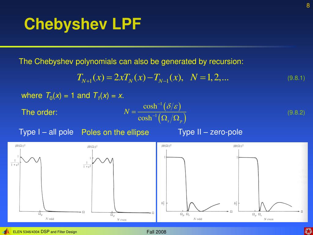
   • This creates exactly $N$ "ripples" (maxima and minima) in the passband from $\omega =0$ to $\omega ={\omega }_p$. The passband ripple in decibels is related to $\epsilon$ by $A_p=10{\log }_{10}(1+{\epsilon }^2)$.

2. Stopband ($\omega >{\omega }_p$):

   • The argument $\omega /{\omega }_p$ is greater than 1.
   • In this range, $T_N(\omega /{\omega }_p)$ increases monotonically and rapidly.
   • This causes the denominator to grow quickly, resulting in a steep, monotonic roll-off in the stopband.

The image below shows the magnitude response for different orders, clearly illustrating the passband ripple and the steeper roll-off compared to a Butterworth filter.

Deriving the Transfer Function $H(s)$

The process is analogous to the Butterworth derivation but with some key differences. We need to find the filter order $N$ and the pole locations.

The following resources provide the complete mathematical derivation. The MIT notes offer a rigorous, step-by-step procedure, while the video offers a highly intuitive way to visualize the pole locations.

Let's summarize the key steps from these resources:

1. Determine Filter Order ($N$): Given passband ripple $A_p$, stopband attenuation $A_s$, passband edge ${\omega }_p$, and stopband edge ${\omega }_s$, we first find $\epsilon$ and another parameter $k_1$ related to the attenuation levels. The required order $N$ is then found using the inverse hyperbolic cosine function:
   $N\ge \frac{{\cosh }^{-1}(\sqrt{k_1})}{{\cosh }^{-1}({\omega }_s/{\omega }_p)}$
   You'll almost always round $N$ up to the next integer. This formula is the Chebyshev equivalent of the logarithm-based formula for the Butterworth order.

2. Find the Pole Locations: As you saw, the poles of a Butterworth filter lie on a circle. For a Chebyshev filter, they lie on an ellipse in the s-plane.

   • The poles of $H(s)H(-s)$ are found by solving $1+{\epsilon }^2{T}_N^2(s/j{\omega }_p)=0$.
   • This derivation, shown in the MIT notes, results in pole locations $s_k={\sigma }_k+j{\Omega }_k$ where:
     ${\sigma }_k=-{\omega }_p\sin \left(\frac{(2k-1)\pi }{2N}\right)\sinh \left(\frac{1}{N}{\sinh }^{-1}\frac{1}{\epsilon }\right)$
     ${\Omega }_k={\omega }_p\cos \left(\frac{(2k-1)\pi }{2N}\right)\cosh \left(\frac{1}{N}{\sinh }^{-1}\frac{1}{\epsilon }\right)$
     for $k=1,2,\dots ,N$. These are the $N$ stable, left-half-plane poles.

3. Construct the Transfer Function $H(s)$:

   • Once you have the $N$ stable poles $p_1,\dots ,p_N$, you form the denominator: $(s-p_1)(s-p_2)\cdots (s-p_N)$.
   • The numerator is a constant chosen to set the DC gain correctly. If $N$ is odd, $T_N(0)=0$ and the DC gain is 1. If $N$ is even, $T_N(0)=\pm 1$ and the DC gain is $1/\sqrt{1+{\epsilon }^2}$. The numerator constant must be adjusted to match this.

3. The Chebyshev Type II Filter: Equiripple Stopband

The Chebyshev Type II, or inverse Chebyshev, filter reverses the roles of the passband and stopband. It offers a maximally flat passband (like Butterworth) but introduces ripples in the stopband. This is achieved by including zeros on the $j\omega$-axis.

Magnitude Response and Analysis

The magnitude-squared response for a Type II filter is:

$|H(j\omega ){|}^2=\frac{1}{1+\frac{1}{{\epsilon }^2{T}_N^2({\omega }_s/\omega )}}$

Notice the key difference: the argument of the Chebyshev polynomial is inverted, ${\omega }_s/\omega$.

• Stopband ($\omega \ge {\omega }_s$): The argument ${\omega }_s/\omega$ is between 0 and 1. This is where $T_N$ oscillates, creating an equiripple stopband. The zeros of the filter occur at frequencies where $T_N^2({\omega }_s/\omega )$ goes to infinity, which physically corresponds to the response dropping to zero. These zeros are located on the $j\omega$-axis and are responsible for the deep nulls in the stopband.
• Passband ($\omega <{\omega }_s$): The argument ${\omega }_s/\omega$ is greater than 1. Here, $T_N$ grows monotonically, causing the second term in the denominator to approach zero quickly, resulting in a flat passband.

Deriving the Transfer Function $H(s)$

The derivation for Type II filters involves finding both poles and zeros.

The key points are:

1. Zeros: The zeros of $H(s)$ lie on the $j\omega$-axis at locations $z_k$ that satisfy $T_N({\omega }_s/z_k)=0$. These are finite-frequency nulls in the stopband.
2. Poles: The poles of a Type II filter are related to the poles of a Type I filter through an inversion. If $p_k^I$ is a pole of a Type I filter, the corresponding Type II pole is $p_k^{II}={\omega }_p{\omega }_s/p_k^I$.
3. Transfer Function: The final transfer function is constructed from both the left-half-plane poles and the zeros on the imaginary axis:
   $H(s)=K\frac{(s-z_1)(s-z_2)\cdots (s-z_M)}{(s-p_1)(s-p_2)\cdots (s-p_N)}$
   where $M<N$ and $K$ is a gain constant to ensure unity gain at DC.

Type II filters are used less often than Type I because for the same order, the roll-off is not as steep, and the introduction of zeros can make the circuit realization more complex. However, they are valuable when a flat passband is critical and stopband ripple is acceptable.

Conclusion

Today we explored the powerful Chebyshev filter approximations, which trade passband flatness for a significantly improved transition bandwidth.

Key Takeaways:

• Chebyshev Polynomials are the mathematical engine of the filter, providing equiripple behavior for $|x|\le 1$ and monotonic behavior for $|x|>1$.
• Type I Filters have an equiripple passband and a monotonic stopband. They are all-pole filters whose poles lie on an ellipse in the s-plane, providing a steeper roll-off than a Butterworth filter of the same order.
• Type II (Inverse) Filters have a monotonic passband and an equiripple stopband. They achieve this using zeros on the $j\omega$-axis, which create nulls in the stopband response.
• The design process for both involves calculating the required filter order $N$ and ripple factor $\epsilon$ from specifications, then determining the pole (and zero) locations to construct the transfer function $H(s)$.

Preview of the Next Lesson:
We've seen two philosophies: maximally flat (Butterworth) and equiripple in one band (Chebyshev). What if we combined them? In our next lesson, we will derive the elliptic (Cauer) filter approximation, which allows for ripple in both the passband and the stopband. This "no-compromise" approach yields the steepest possible roll-off for any given filter order, representing the pinnacle of classical filter design efficiency.