Transfer Function to Frequency Response

1. The s-Plane and the jω-Axis: A Conceptual Bridge

Before diving into the formal mathematics, let's build a strong conceptual link between the Laplace and Fourier transforms. Your background in signal processing has given you a solid foundation in both, and seeing them as parts of a greater whole is enlightening.

The Laplace transform variable is a complex frequency $s=\sigma +j\omega$. The term $e^{-st}=e^{-\sigma t}{e}^{-j\omega t}$ acts as a probe. It analyzes a function's content in terms of both pure sinusoids ($e^{-j\omega t}$) and exponentially decaying or growing sinusoids ($e^{-\sigma t}$). The resulting transform $F(s)$ exists on a two-dimensional complex plane, the s-plane.

The Fourier transform, on the other hand, only uses pure sinusoids ($e^{-j\omega t}$) as its basis. This is equivalent to setting the real part of the complex frequency, $\sigma$, to zero. In other words, the Fourier transform is a special case of the bilateral Laplace transform where $s=0+j\omega$, confined to the imaginary axis of the s-plane.

This video offers an excellent visualization of this very concept.

This visualization suggests that all the information about a system's response to pure sinusoids should be contained within its transfer function $H(s)$ right on the $j\omega$ axis. Now, let's prove this rigorously.

2. The Formal Derivation: From H(s) to Steady-State Response

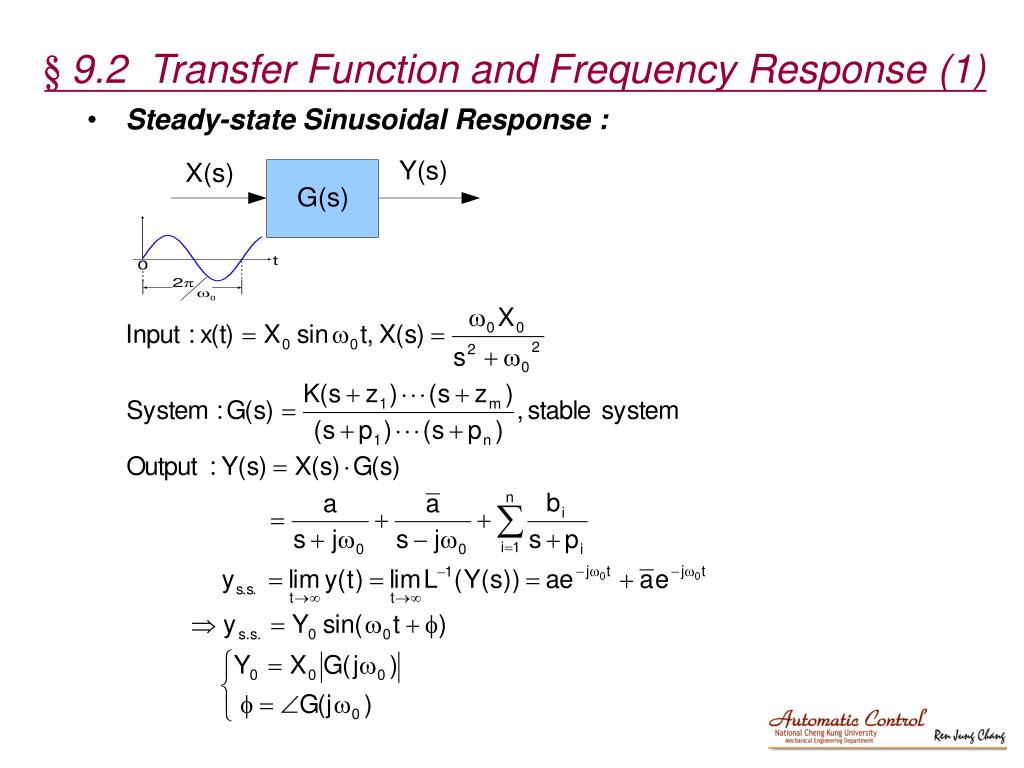
Our objective is to prove that for a stable LTI system with transfer function $H(s)$ and a sinusoidal input $x(t)=A\cos ({\omega }_{0}t)$, the steady-state output will be $y_{ss}(t)=A|H(j{\omega }_0)|\cos ({\omega }_{0}t+\angle H(j{\omega }_0))$.

This derivation is a classic piece of signals and systems analysis. The following resource provides a step-by-step mathematical argument that we will replicate and explain here.

Let's proceed with the derivation, step-by-step.

Step 1: Define the Input and System in the s-Domain

• System: A stable, linear time-invariant (LTI) system is characterized by its transfer function $H(s)=Y(s)/X(s)$, where we assume all initial conditions are zero.
• Input: We consider a general sinusoidal input, $x(t)=A\cos ({\omega }_{0}t)$. Using Euler's formula, we can write this in a form more suitable for Laplace transformation:
  $x(t)=\frac{A}{2}(e^{j{\omega }_{0}t}+e^{-j{\omega }_{0}t})$
• Input Transform: Using the standard transform pair $\mathcal{L}\{e^{at}\}=\frac{1}{s-a}$, the Laplace transform of the input is:
  $X(s)=\frac{A}{2}\left(\frac{1}{s-j{\omega }_0}+\frac{1}{s+j{\omega }_0}\right)$

Step 2: Determine the Output Transform Y(s)

The output transform $Y(s)$ is simply the product of the input transform and the system's transfer function:
$Y(s)=H(s)X(s)=H(s)\cdot \frac{A}{2}\left(\frac{1}{s-j{\omega }_0}+\frac{1}{s+j{\omega }_0}\right)$

To find the time-domain output $y(t)$, we must find the inverse Laplace transform of $Y(s)$. This requires a partial fraction expansion. The poles of $Y(s)$ come from two sources:

1. The poles of the input, at $s=j{\omega }_0$ and $s=-j{\omega }_0$.
2. The poles of the system, which are the roots of the denominator of $H(s)$. Let's call these $p_1,p_2,\dots ,p_n$.

The partial fraction expansion will therefore have the form:
$Y(s)=\underset{\text{Terms from input poles}}{\underbrace{\frac{C}{s-j{\omega }_0}+\frac{C^{\ast }}{s+j{\omega }_0}}}+\underset{\text{Terms from system poles}}{\underbrace{\sum _{k=1}^n\frac{R_k}{s-p_k}}}$
(Note: The second coefficient must be the complex conjugate $C^{\ast }$ because the time-domain signal $y(t)$ is real.)

Step 3: Isolate the Steady-State Response

The inverse Laplace transform of the full expression for $Y(s)$ gives the total response:
$y(t)=\underset{\text{Forced / Steady-State Response}}{\underbrace{C{e}^{j{\omega }_{0}t}+C^{\ast }{e}^{-j{\omega }_{0}t}}}+\underset{\text{Natural / Transient Response}}{\underbrace{\sum _{k=1}^n{R}_k{e}^{p_{k}t}}}$

Here is where the stability of the system is critical. For a stable system, all of its poles $p_k$ lie in the left half of the s-plane, meaning $\text{Re}\{p_k\}<0$ for all $k$. Consequently, every term in the natural response, $R_k{e}^{p_{k}t}$, contains a decaying exponential factor and will approach zero as $t\to \infty$.

The frequency response specifically describes the sinusoidal steady-state behavior of the system, which is what remains after all transients have died out. Therefore, we are only interested in the first two terms:
$y_{ss}(t)=C{e}^{j{\omega }_{0}t}+C^{\ast }{e}^{-j{\omega }_{0}t}$

Step 4: Calculate the Coefficient C

To find $y_{ss}(t)$, we just need to find the complex coefficient $C$. We can do this using the Heaviside cover-up method for partial fraction expansion:
$C={\left[(s-j{\omega }_0)Y(s)\right]}_{s=j{\omega }_0}$
Substituting the expression for $Y(s)$:
$C={\left[(s-j{\omega }_0)\cdot H(s)\cdot \frac{A}{2}\left(\frac{1}{s-j{\omega }_0}+\frac{1}{s+j{\omega }_0}\right)\right]}_{s=j{\omega }_0}$
Distributing the $(s-j{\omega }_0)$ term inside the parenthesis:
$C={\left[H(s)\cdot \frac{A}{2}\left(1+\frac{s-j{\omega }_0}{s+j{\omega }_0}\right)\right]}_{s=j{\omega }_0}$
Now, we evaluate this expression by setting $s=j{\omega }_0$. The fractional term becomes zero.
$C=H(j{\omega }_0)\cdot \frac{A}{2}\left(1+\frac{j{\omega }_0-j{\omega }_0}{j{\omega }_0+j{\omega }_0}\right)=H(j{\omega }_0)\cdot \frac{A}{2}$

Step 5: Reconstruct the Time-Domain Output

Now we substitute this result for $C$ back into our expression for $y_{ss}(t)$. The complex value $H(j{\omega }_0)$ can be represented in polar form as:
$H(j{\omega }_0)=|H(j{\omega }_0)|e^{j\angle H(j{\omega }_0)}$
Let's denote the phase $\varphi ({\omega }_0)=\angle H(j{\omega }_0)$. Then $C=\frac{A}{2}|H(j{\omega }_0)|e^{j\varphi ({\omega }_0)}$ and its conjugate is $C^{\ast }=\frac{A}{2}|H(j{\omega }_0)|e^{-j\varphi ({\omega }_0)}$.

Substituting these into the equation for $y_{ss}(t)$:
$y_{ss}(t)=\left(\frac{A}{2}|H(j{\omega }_0)|e^{j\varphi ({\omega }_0)}\right)e^{j{\omega }_{0}t}+\left(\frac{A}{2}|H(j{\omega }_0)|e^{-j\varphi ({\omega }_0)}\right)e^{-j{\omega }_{0}t}$
Factoring out the common terms:
$y_{ss}(t)=A|H(j{\omega }_0)|\left(\frac{e^{j({\omega }_{0}t+\varphi ({\omega }_0))}+e^{-j({\omega }_{0}t+\varphi ({\omega }_0))}}{2}\right)$
The expression in the parentheses is simply the definition of cosine. This gives us our final, powerful result:
$y_{ss}(t)=A|H(j{\omega }_0)|\cos ({\omega }_{0}t+\varphi ({\omega }_0))$

This derivation proves that the steady-state output of a stable LTI system to a sinusoidal input is also a sinusoid of the same frequency, but with its amplitude multiplied by $|H(j{\omega }_0)|$ and its phase shifted by $\angle H(j{\omega }_0)$.

The complex function $H(j\omega )$ completely defines this relationship for all frequencies and is therefore rightfully called the frequency response function.

The image below provides a concise summary of this entire derivation.

Conclusion

Today we have rigorously proven one of the most useful results in LTI system theory. By starting with a sinusoidal input and tracing its path through the system using Laplace transforms, we have formally derived the direct relationship between the s-domain transfer function and the frequency-domain response.

Key Takeaways:

• The frequency response $H(j\omega )$ is not just a convenient notation; it is the transfer function $H(s)$ evaluated at $s=j\omega$, and this substitution is mathematically justified.
• The derivation relies on a partial fraction expansion of the output $Y(s)$, separating it into transient terms (from system poles) and steady-state terms (from input poles).
• For a stable system, the transient terms decay to zero, leaving a purely sinusoidal steady-state response.
• The magnitude of the frequency response, $|H(j\omega )|$, gives the gain (amplitude ratio) of the system at frequency $\omega$.
• The phase of the frequency response, $\angle H(j\omega )$, gives the phase shift added by the system at frequency $\omega$.

Preview of the Next Lesson:
Now that we have firmly established the link between $H(s)$ and $H(j\omega )$, we can focus on analyzing the frequency response itself. In the next lesson, we will delve into the characteristics of analog filters by examining their magnitude response, phase response, and a related concept called group delay. This will allow us to understand and predict how a system will shape signals in the frequency domain, a critical skill for filter design and analysis.