DTFT Periodicity and Its Implications

1. The Mathematical Root of Periodicity

The periodicity of the DTFT, $X(e^{j\omega })$, arises directly from the properties of the complex exponential function with an integer index. Let's start with the definition of the DTFT:

The key is the term $e^{-j\omega n}$, where $n$ is always an integer. Let's see what happens if we shift the frequency $\omega$ by an integer multiple of $2\pi$, say $\omega +2\pi k$ for some integer $k$.

The following video provides a concise mathematical proof of this property.

As the video demonstrates, if we substitute $\omega +2\pi k$ into the complex exponential term, we get:

Using Euler's formula, the second term becomes:

Since both $k$ and $n$ are integers, their product $kn$ is also an integer. The cosine of an integer multiple of $2\pi$ is always 1, and the sine is always 0. Therefore, $e^{-j2\pi kn}=1$.

This proves that $e^{-j(\omega +2\pi k)n}=e^{-j\omega n}$ for any integer $k$. When we substitute this back into the DTFT summation, it shows that the entire transform is periodic with period $2\pi$:

This intrinsic property distinguishes the DTFT from its continuous-time counterpart, which is generally aperiodic.

2. The Physical Origin of Periodicity: The Act of Sampling

While the direct proof shows that the DTFT is periodic, the relationship we derived in the last lesson explains why it becomes periodic: the process of sampling itself.

As a brief recap, sampling a continuous signal $s(t)$ at intervals of $T$ creates a discrete sequence $s[n]=s(nT)$. The spectrum of this discrete sequence, its DTFT, is directly related to the spectrum of the original continuous signal, $S(f)$, through the Poisson summation formula. This formula provides a beautifully complete picture.

The Poisson summation formula (Eq. 2 in the article) states:

This equation tells us that the DTFT spectrum ($S_{1/T}(f)$ in this notation) is not a new, unrelated entity. It is literally constructed by taking the original continuous-time spectrum $S(f)$, making infinite copies of it, and shifting each copy by an integer multiple of the sampling frequency, $f_s=1/T$.

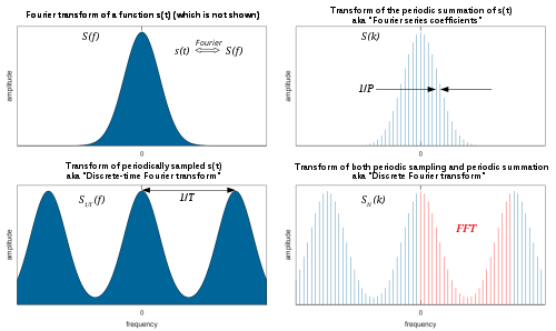
This figure from the Wikipedia article illustrates the creation of the periodic DTFT spectrum (bottom left) from the aperiodic CTFT spectrum (top left) through the process of sampling. The spacing of the spectral replicas is determined by the sampling frequency.

This process of "periodic summation" naturally creates a periodic function. This is the physical and conceptual reason behind the mathematical property we proved earlier. The discrete nature of the time-domain signal $x[n]$ forces its frequency-domain representation to be continuous and periodic.

3. Key Implications of Periodicity

The $2\pi$-periodicity of the DTFT spectrum is not just a theoretical detail; it has profound practical consequences that shape the entire field of digital signal processing.

a) Redundancy and the Unique Frequency Range

Since the spectrum repeats every $2\pi$ radians/sample, all the unique information about the signal's frequency content is contained within any single interval of length $2\pi$. By convention, we typically analyze the principal period from $\omega =-\pi$ to $\omega =\pi$. The spectrum outside this range is entirely redundant.

This leads to a different interpretation of "low" and "high" frequencies compared to the continuous-time domain:

• Low Frequencies: Frequencies near integer multiples of $2\pi$ (e.g., $\omega \approx 0,\pm 2\pi ,\dots$) correspond to slowly varying signals.
• High Frequencies: Frequencies near odd integer multiples of $\pi$ (e.g., $\omega \approx \pm \pi ,\pm 3\pi ,\dots$) correspond to rapidly varying signals. The highest unique frequency in a discrete-time signal occurs at $\omega =\pi$.

b) Aliasing: The Problem of Ambiguity

The most critical implication of periodicity is aliasing. Because $X(e^{j\omega })=X(e^{j(\omega +2\pi k)})$, it is impossible to distinguish between the frequency $\omega$ and any of its aliases $\omega \pm 2\pi$, $\omega \pm 4\pi$, etc., based on the sampled signal alone.

Let's connect this back to the continuous world. A continuous frequency $\Omega$ maps to the discrete frequency $\omega =\Omega T_s$. Now consider a higher continuous frequency ${\Omega }^{\prime }=\Omega +{\Omega }_s$, where ${\Omega }_s=2\pi /T_s$ is the sampling frequency. Its corresponding discrete frequency is:

After sampling, the continuous frequency $\Omega +{\Omega }_s$ is indistinguishable from $\Omega$. It has taken on the "alias" of the lower frequency. This is the phenomenon you observed in the exercise from the previous lesson, now explained through the structure of the DTFT.

This next video excellently illustrates how the periodic replication of the spectrum leads to aliasing if the sampling rate is not high enough.

c) The Nyquist-Shannon Sampling Theorem Revisited

The problem of aliasing leads directly to its solution: the Nyquist-Shannon sampling theorem. The video you just watched explained it visually. The periodic nature of the DTFT demands that if we want to be able to perfectly reconstruct the original signal, the spectral copies created by sampling must not overlap.

For a signal band-limited to $|\Omega |<{\Omega }_{\text{max}}$, its spectral width is $2{\Omega }_{\text{max}}$. The copies are centered at integer multiples of the sampling frequency ${\Omega }_s$. To prevent overlap, the distance between the centers of adjacent copies (${\Omega }_s$) must be greater than the width of one copy ($2{\Omega }_{\text{max}}$).

This is the famous Nyquist criterion, derived here as a direct consequence of avoiding the spectral overlap inherent in the DTFT's periodic structure.

Conclusion

In this lesson, we took a deep dive into the periodicity of the DTFT. You saw how this fundamental property is both a direct mathematical consequence of the DTFT's definition and a physical consequence of the spectral replication caused by sampling.

Key Takeaways:

• The DTFT spectrum $X(e^{j\omega })$ is always periodic with period $2\pi$, because the complex exponential kernel $e^{-j\omega n}$ is itself periodic in $\omega$ for integer $n$.
• Conceptually, this periodicity arises from the fact that sampling in the time domain creates infinite, uniformly-spaced replicas of the original signal's spectrum in the frequency domain.
• Implication 1: All unique frequency information is contained in the principal period, typically $[-\pi ,\pi ]$.
• Implication 2: Periodicity causes frequency ambiguity, or aliasing, where continuous frequencies separated by multiples of the sampling frequency ($f_s$) become indistinguishable after sampling.
• Implication 3: The Nyquist-Shannon sampling theorem ($f_s>2f_{\text{max}}$) is the condition required to prevent the periodic spectral replicas from overlapping and causing aliasing.

Preview of the Next Lesson:

Having thoroughly analyzed the DTFT and its properties, we are now ready to generalize it. In the next lesson, we will derive the z-transform as a generalization of the DTFT. You will see that while the DTFT is confined to analyzing frequencies on the unit circle in the complex plane, the z-transform allows us to analyze the entire plane, providing powerful tools for understanding system stability and causality.