Z-Plane Unit Circle and DTFT Frequency Response

1. The Mathematical Connection: Evaluating the Z-Transform on the Unit Circle

Let's begin by solidifying the mathematical link we introduced last time. The definitions for the z-transform of a system's impulse response, $h[n]$, and its DTFT are:

• Z-Transform: $H(z)={\sum }_{n=-\infty }^{\infty }h[n]z^{-n}$
• DTFT (Frequency Response): $H(e^{j\omega })={\sum }_{n=-\infty }^{\infty }h[n]e^{-j\omega n}$

It's clear from these equations that if we take the z-transform expression $H(z)$ and substitute the complex variable $z$ with $e^{j\omega }$, we get the DTFT.

The following short video provides an excellent summary of this exact point.

2. The Geometry of Frequency: The Unit Circle

The substitution $z=e^{j\omega }$ has a profound geometric meaning. A general complex number in the z-plane can be written in polar form as $z=r{e}^{j\omega }$, where $r$ is the magnitude (distance from the origin) and $\omega$ is the angle (in radians) from the positive real axis.

When we set $z=e^{j\omega }$, we are fixing the magnitude to $r=1$. The set of all complex numbers with a magnitude of 1 forms the unit circle.

This mapping directly connects discrete-time frequency $\omega$ to a physical location on the z-plane:

• DC ($\omega =0$): This corresponds to $z=e^{j0}=1$, the point on the far right of the unit circle.
• Nyquist Frequency ($\omega =\pi$): This corresponds to $z=e^{j\pi }=-1$, the point on the far left of the unit circle.
• Negative Nyquist Frequency ($\omega =-\pi$): This also corresponds to $z=e^{-j\pi }=-1$. Moving clockwise from $z=1$ represents negative frequencies.
• Full Cycle ($\omega =2\pi$): This corresponds to $z=e^{j2\pi }=1$, bringing us back to where we started. This journey around the circle is a beautiful geometric confirmation of the $2\pi$-periodicity of the DTFT we studied earlier.

The following reading reinforces these points clearly.

3. Visualizing the Frequency Response

Now, let's combine these ideas. The magnitude of the z-transform, $|H(z)|$, can be visualized as a 3D surface plotted over the complex z-plane. The value of $|H(z)|$ is the height of the surface at the point $z$.

This surface is shaped by the poles and zeros of $H(z)$:

• At a pole, the function goes to infinity, so the surface has an infinitely high peak.
• At a zero, the function is zero, so the surface touches the z-plane.

The DTFT magnitude response, $|H(e^{j\omega })|$, is simply the cross-section of this 3D surface along the unit circle.

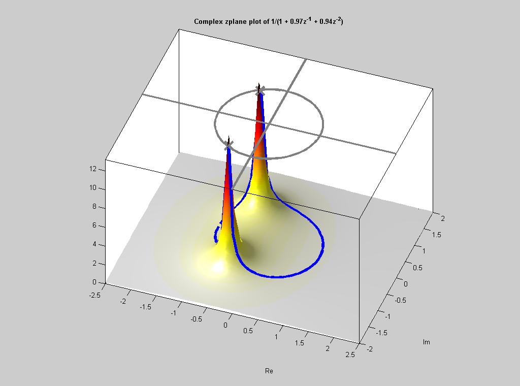
This visualization provides powerful intuition:

• If a pole is located close to the unit circle, the frequency response will have a sharp peak at the frequency $\omega$ corresponding to the pole's angle. The closer the pole is to the circle, the higher and sharper the peak.
• If a zero is located on or near the unit circle, the frequency response will have a null or dip at the corresponding frequency $\omega$.

This geometric relationship is the foundation of analog and digital filter design, where poles and zeros are carefully placed to shape the frequency response of a system.

To see another perspective on this visualization, consider the following video.

4. Stability, ROC, and the Existence of a Frequency Response

We can now bring everything together. As you know from your background in continuous-time systems, a stable LTI system has an impulse response $h(t)$ that is absolutely integrable. The discrete-time equivalent is that a stable system has an impulse response $h[n]$ that is absolutely summable:

If this condition holds, then the DTFT sum is guaranteed to converge, because:

This ties directly back to the z-transform and the ROC. For the DTFT to exist, the z-transform sum must converge for $z=e^{j\omega }$, i.e., on the unit circle. This leads to a fundamental conclusion:

An LTI system is stable if and only if the ROC of its transfer function $H(z)$ includes the unit circle.

The following readings formalize this critical link between the abstract ROC and the practical concepts of stability and frequency response.

Conclusion

In this lesson, we established a robust and intuitive link between the z-plane and the frequency domain. By understanding the z-transform as a surface and the DTFT as a slice of that surface, you've gained a powerful tool for analyzing system behavior.

Key Takeaways:

• The DTFT of a signal is mathematically equivalent to its z-transform evaluated on the unit circle ($z=e^{j\omega }$).
• Discrete-time frequency $\omega$ corresponds to the angle on the unit circle, with $\omega =0$ at $z=1$ and $\omega =\pi$ at $z=-1$.
• The magnitude of the frequency response, $|H(e^{j\omega })|$, can be visualized as the cross-section of the 3D surface $|H(z)|$ along the unit circle.
• Poles near the unit circle create peaks in the frequency response, while zeros create nulls. This proximity effect is the key to filter design.
• A system's frequency response exists and the system is stable if and only if the ROC of its z-transform, $H(z)$, includes the unit circle.

Preview of the Next Lesson:

Having established the fundamental concepts of the z-transform, the ROC, and the link to frequency response, we are now ready to put it to work. In the next lesson, we will explore the key properties of the z-transform (linearity, shift, convolution, etc.). This will give us the analytical machinery needed to efficiently analyze and solve problems involving discrete-time LTI systems, much as we did with Laplace transform properties for continuous-time systems.