Z-Plane Analysis: Stability and Causality

Hello! Welcome back to our study of discrete-time systems.

In the last lesson, we established a powerful workflow: starting with a system's difference equation, we used the properties of the z-transform to derive its algebraic equivalent—the transfer function, $H (z)$ . We saw that this function, a ratio of polynomials in $z$ , neatly encapsulates the system's input-output behavior.

Today, we will address the crucial question of what the transfer function tells us about the fundamental nature of the system. Our goal is to analyze the stability and causality of discrete-time systems using pole-zero locations in the z-plane. By simply looking at where the poles of $H (z)$ lie relative to the unit circle, we can determine if a system is stable and causal, without ever needing to calculate an inverse transform or simulate its response. This is one of the most elegant and practical aspects of z-domain analysis.

1. The Role of the Region of Convergence (ROC)

Before we dive into stability and causality, let's briefly revisit a concept that links them: the Region of Convergence (ROC). As we've discussed, the z-transform of a sequence is not uniquely defined by its algebraic expression alone; we also need the ROC. The shape of the ROC is directly tied to the nature of the time-domain signal.

Let's quickly review the key relationships:

Causal (Right-Sided) Signals: A signal $h [n]$ that is zero for $n < 0$ has an ROC that is the exterior of a circle in the z-plane, extending to $z = \infty$ . The radius of this circle is determined by the magnitude of the outermost pole.
Anti-Causal (Left-Sided) Signals: A signal $h [n]$ that is zero for $n > - 1$ has an ROC that is the interior of a circle in the z-plane.
Two-Sided Signals: A signal with non-zero values for both positive and negative $n$ has an annular (ring-shaped) ROC, bounded by poles.

This connection is fundamental because causality is a property of the impulse response $h [n]$ , and the ROC of $H (z)$ is determined by the properties of $h [n]$ .

To refresh your memory on how these ROCs are derived, you might find it helpful to review parts of this video we've touched on before.

Region of Convergence for the z-Transform

This clip from Barry Van Veen's 'Region of Convergence for the z-Transform' video quickly reviews the derivation of the ROC for both causal and anti-causal exponential signals, which form the building blocks of any impulse response.

If you need a refresher, watch from 02:16 to 09:33. Focus on how a causal signal leads to an ROC of the form |z| > |α| and an anti-causal signal leads to an ROC of |z| < |α|.

2. Causality and Stability in the Z-Domain

With the ROC properties in mind, we can now establish formal conditions for causality and stability. Let's consider an LTI system with a rational transfer function $H (z)$ .

Causality Condition

A system is causal if its impulse response $h [n]$ is zero for all $n < 0$ . As we just reviewed, this means $h [n]$ is a right-sided sequence. For a rational $H (z)$ , this implies a specific structure for the ROC.

A discrete-time LTI system with a rational transfer function $H (z)$ is causal if and only if its ROC is the exterior of a circle that includes $z = \infty$ . This means the ROC is of the form $∣ z ∣ > ∣ p_{ma x} ∣$ , where $p_{ma x}$ is the pole with the largest magnitude.

Another way to state this for rational functions is that the order of the numerator polynomial cannot be greater than the order of the denominator polynomial. If it were, long division would yield positive powers of $z$ , corresponding to time-domain components at $n < 0$ .

Stability Condition

A system is Bounded-Input, Bounded-Output (BIBO) stable if every bounded input produces a bounded output. For LTI systems, this is equivalent to the impulse response being absolutely summable:
$\sum_{n = - \infty}^{\infty} ∣ h [n] ∣ < \infty$
This condition has a direct and profound implication for the z-transform. Recall that the Discrete-Time Fourier Transform (DTFT), $H (e^{j ω})$ , which represents the system's frequency response, is simply the z-transform evaluated at $z = e^{j ω}$ . The DTFT integral (or sum) converges only if the signal is absolutely summable.

Therefore, for a stable system, the z-transform must converge on the unit circle.

A discrete-time LTI system is BIBO stable if and only if the ROC of its transfer function $H (z)$ includes the unit circle, $∣ z ∣ = 1$ .

The following video provides a clear derivation of this crucial result.

Stability and Causality of LTI Systems Described by Difference Equations

In this video, 'Stability and Causality of LTI Systems' by Barry Van Veen, the presenter formally derives the stability condition from the absolute summability of the impulse response.

Please watch from 03:29 to 05:52. Pay close attention to how the triangle inequality is used to show that \sum |h[n]| being finite implies that |H(z)| must be bounded when evaluated on the unit circle.

3. Combining Causality and Stability

Now we can combine these two conditions to find the requirement for a system to be both causal and stable—the most desirable case for many real-world applications.

For causality, the ROC must be outside the outermost pole: $∣ z ∣ > ∣ p_{ma x} ∣$ .
For stability, the ROC must include the unit circle, $∣ z ∣ = 1$ .

For both to be true, the unit circle must lie within the region $∣ z ∣ > ∣ p_{ma x} ∣$ . This can only happen if the outermost pole itself is inside the unit circle, i.e., $∣ p_{ma x} ∣ < 1$ .

A causal LTI system with a rational transfer function $H (z)$ is stable if and only if all of its poles lie inside the unit circle.

This is a cornerstone principle of digital signal processing. The location of the poles tells you everything you need to know about the system's stability.

This rule makes intuitive sense when we visualize the pole locations and their corresponding impulse responses.

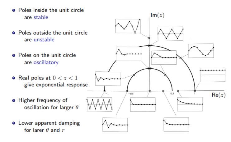
Z-Plane Pole Response Characteristics — This diagram illustrates how the location of a pole in the z-plane determines the time-domain behavior of the system's impulse response. Poles inside the unit circle lead to decaying (stable) responses, while poles outside lead to growing (unstable) responses. Poles on the unit circle result in sustained (marginally stable) oscillations.

The reason the unit circle is the stability boundary is directly related to the mapping from the s-plane, which you are familiar with from continuous-time control systems.

Z-Transform & Pole-Zero Distribution & Stability Considerations — This image shows the mapping $z = e^{sT}$. The stable left-half of the s-plane ($\\text{Re}(s) < 0$) maps to the interior of the unit circle in the z-plane ($|z| < 1$), while the imaginary axis ($\\text{Re}(s) = 0$) maps to the unit circle itself ($|z| = 1$).

What if Stability and Causality are Incompatible?

Consider a system with poles both inside and outside the unit circle. For example, poles at $z = 0.5$ and $z = 2$ .

To be causal, the ROC must be $∣ z ∣ > 2$ . This region does not include the unit circle, so the system is unstable.
To be stable, the ROC must include the unit circle. The only possible ROC that does this is the annular region $0.5 < ∣ z ∣ < 2$ . Since this ROC is not the exterior of the outermost pole, the corresponding impulse response is two-sided and thus non-causal.

In this case, you can have a causal system or a stable system, but not both. The following video segment works through this exact scenario.

Stability and Causality of LTI Systems Described by Difference Equations

Let's return to the video 'Stability and Causality of LTI Systems' to see a concrete example of analyzing a system where stability and causality are mutually exclusive.

Watch from 01:54 to 08:58. This segment first states the causality condition, then works through an example of a system with poles at z=2 and z=-0.5. Notice how choosing a causal ROC leads to an unstable system, and choosing a stable ROC leads to a non-causal system. The segment concludes by stating the combined condition for causal and stable systems.

Test your understanding!

An LTI system has the transfer function:

H (z) = \frac{z}{( z - 0.8 ) ( z - 1.2 )}

The system is known to be stable. Is it causal? What is its ROC?

Show answer

Identify Poles: The poles are at $p_{1} = 0.8$ and $p_{2} = 1.2$ .
Apply Stability Condition: Since the system is stable, its ROC must include the unit circle ( $∣ z ∣ = 1$ ).
Determine ROC: The possible ROCs are bounded by the poles: $∣ z ∣ < 0.8$ , $0.8 < ∣ z ∣ < 1.2$ , and $∣ z ∣ > 1.2$ . The only one of these regions that contains the unit circle is the annular region $0.8 < ∣ z ∣ < 1.2$ . This must be the system's ROC.
Check Causality: A causal system would have an ROC of $∣ z ∣ > 1.2$ (outside the outermost pole). Since our ROC is $0.8 < ∣ z ∣ < 1.2$ , the system is not causal. The impulse response will be two-sided, with the pole at 0.8 contributing a causal part and the pole at 1.2 contributing an anti-causal part.

4. Marginal Stability and the Role of Zeros

Marginal Stability: What if poles lie exactly on the unit circle?

If a system has non-repeated (distinct) poles on the unit circle and all other poles are inside, the system is considered marginally stable. Its impulse response will not decay to zero but will remain bounded (e.g., a pure sinusoid). An example is a pole at $z = e^{j ω_{0}}$ , which creates an everlasting oscillation at frequency $ω_{0}$ . Note that the impulse response is not absolutely summable, so such a system is not strictly BIBO stable.
If a system has repeated poles on the unit circle (e.g., two poles at $z = 1$ ), the system is unstable. The response will grow over time (e.g., $n (1)^{n} u [n]$ which is a ramp).

The Role of Zeros:
Poles determine the system's natural modes and thus its stability. Zeros do not affect stability. Instead, they shape the frequency response by creating nulls. A zero at a certain frequency $z_{0} = e^{j ω_{0}}$ means the system will completely block any input at that frequency.

An important subtlety arises with pole-zero cancellation. If a system has an unstable pole that is canceled by a zero at the same location, the system may appear stable from an input-output perspective (BIBO stable), but it is not internally stable. The unstable mode still exists within the system but is hidden from the output. This is a key concept in control theory.

For a more formal treatment of these ideas, the following text provides excellent, concise definitions.

Stability of Discrete-time systems

For a clear summary of these stability criteria, please refer to the document 'Stability of Discrete-time systems' by F.L. Lewis.

Please read pages 1-2 and the summary table on page 5. Focus on the definitions for Asymptotically Stable (AS) and Marginally Stable (MS) systems and how they relate to pole locations. The distinction made between internal stability (all system poles) and BIBO stability (poles of the transfer function after cancellation) is particularly relevant.

Conclusion

Today we've established one of the most powerful analysis tools in DSP. By inspecting a system's pole-zero plot, we can immediately deduce its fundamental characteristics of causality and stability.

Key Takeaways:

Causality implies the ROC is outside the outermost pole ( $∣ z ∣ > ∣ p_{ma x} ∣$ ).
BIBO Stability implies the ROC includes the unit circle ( $∣ z ∣ = 1$ ).
A causal and stable LTI system must have all its poles strictly inside the unit circle.
Poles on the unit circle lead to marginal stability if they are distinct, and instability if they are repeated.
Zeros shape the frequency response but do not determine stability.

Preview of the Next Lesson:

We've mastered how to analyze stability in the z-plane. The next logical question is: how do we design a stable discrete-time system that mimics a known stable analog system? In the next lesson, we will "Derive the relationship between the s-plane poles of an analog system and the z-plane poles of its discrete-time counterpart via impulse invariance." This will be our first step into the practical world of digital filter design, bridging the continuous and discrete domains.

Recommended resources