Heisenberg's Uncertainty Principle and the STFT

1. The Uncertainty Principle: An Intuitive Start

Before diving into the mathematics, let's build an intuition for the core idea. The concept that you can't simultaneously know "when" and "what frequency" with perfect precision is something you already experience.

As the video explains, a short event (like a clap) is ambiguous in frequency, while a pure tone requires a long duration to be identified precisely. The Fourier transform is the mathematical tool that makes this relationship explicit:

• A signal that is compact or highly localized in the time domain will have a Fourier transform that is spread out in the frequency domain.
• Conversely, a signal that is compact or highly localized in the frequency domain (like a pure sine wave) must be spread out in the time domain.

The video also touches on a practical application in Doppler radar, which is a great analogy from your field of electrical engineering. Determining an object's precise location requires a short, sharp pulse, but this makes its velocity (related to frequency via the Doppler shift) uncertain. Conversely, determining precise velocity requires a long pulse, which makes its exact location ambiguous. This is the same fundamental trade-off.

2. Quantifying "Spread": The Time-Bandwidth Product

To move from intuition to a formal principle, we need to mathematically define the "spread" or "duration" of a signal in both time and frequency. A common and powerful way to do this is by using the concept of variance, similar to how it's used in probability and random processes.

For a signal $f(t)$ that is centered at $t=0$ and has unit energy $({\int }_{-\infty }^{\infty }|f(t){|}^{2}dt=1)$, we can define its effective duration and bandwidth as follows:

• The time spread (or RMS duration) ${\sigma }_t$ is the standard deviation of the signal's energy distribution in time:
  ${\sigma }_t^2={\int }_{-\infty }^{\infty }{t}^2|f(t){|}^{2}dt$

• The frequency spread (or RMS bandwidth) ${\sigma }_u$ is the standard deviation of its energy distribution in frequency, where $u$ is frequency in Hertz (Hz):
  ${\sigma }_u^2={\int }_{-\infty }^{\infty }{u}^2|\hat{f}(u){|}^{2}du$
  Here, $\hat{f}(u)$ is the Fourier Transform of $f(t)$.

These two quantities are not independent. They are linked by the Heisenberg Uncertainty Principle for Fourier transforms.

As stated in the notes, the principle is the inequality:
${\sigma }_t^2\cdot {\sigma }_u^2\ge \frac{1}{16{\pi }^2}$
Taking the square root of both sides gives us the relationship between the RMS duration and RMS bandwidth:
${\sigma }_t\cdot {\sigma }_u\ge \frac{1}{4\pi }$

Often in signal processing, we work with angular frequency $\omega =2\pi u$. Since ${\sigma }_{\omega }=2\pi {\sigma }_u$, we can substitute this into the inequality to get the more common form:
${\sigma }_t\cdot {\sigma }_{\omega }\ge \frac{1}{2}$

This is a profound result. It states that the product of a signal's effective duration and its effective bandwidth (often called the time-bandwidth product) has a fixed lower bound. No signal can be arbitrarily narrow in both the time and frequency domains simultaneously.

3. The Uncertainty Principle in the STFT

How does this general principle apply specifically to the STFT? In the previous lesson, we saw that the STFT calculates the spectrum of a windowed portion of the signal. The properties of the STFT are therefore not determined by the signal itself, but by the window function $w(t)$.

• The time resolution of the STFT is determined by the duration of the window function, ${\sigma }_t$ of $w(t)$. A narrower window gives better time resolution.
• The frequency resolution of the STFT is determined by the bandwidth of the window function's Fourier transform, ${\sigma }_{\omega }$ of $W(\omega )$. A narrower spectrum for the window gives better frequency resolution.

The uncertainty principle applies directly to the window function $w(t)$: ${\sigma }_{t,w}\cdot {\sigma }_{\omega ,W}\ge \frac{1}{2}$.
This means that when you design your STFT:

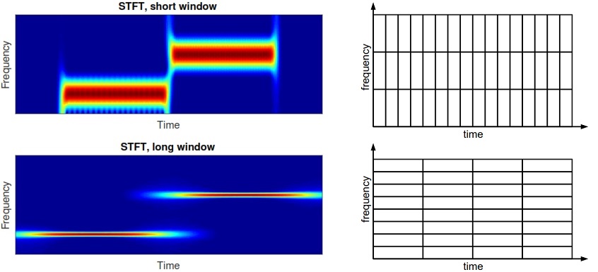
• If you choose a window $w(t)$ that is very narrow in time (small ${\sigma }_{t,w}$), its Fourier transform $W(\omega )$ must be wide (large ${\sigma }_{\omega ,W}$). This gives good time resolution but poor frequency resolution.
• If you choose a window $w(t)$ whose transform $W(\omega )$ is very narrow in frequency (small ${\sigma }_{\omega ,W}$), the window itself must be wide in time (large ${\sigma }_{t,w}$). This gives good frequency resolution but poor time resolution.

This is precisely the trade-off we observed in the last lesson, but now we see it as a direct consequence of a fundamental mathematical limit.

The following image perfectly visualizes this concept by showing how the time-frequency plane is "tiled" by the STFT. The area of each "tile" represents the time-bandwidth product of the window, which is constant.

4. The Optimal Window: The Gaussian Function

The uncertainty principle ${\sigma }_t{\sigma }_{\omega }\ge \frac{1}{2}$ is an inequality. This implies that some functions are more "efficient" than others in packing their energy. This raises a natural question: does any function achieve the theoretical minimum?

The answer is yes. The Gaussian function is unique in that it is the only function that satisfies the uncertainty principle with equality:
${\sigma }_t{\sigma }_{\omega }=\frac{1}{2}$
This means a Gaussian window provides the best possible simultaneous localization in both time and frequency that the uncertainty principle allows. No other window shape can achieve a smaller time-bandwidth product.

This special property is why the Gaussian function is central to time-frequency analysis. In fact, this is precisely what Dennis Gabor used in his pioneering 1946 paper where he introduced this transform, which is why the STFT is often called the Gabor Transform.

The connection to quantum mechanics mentioned in the last clip is not accidental. The Heisenberg uncertainty principle in quantum mechanics, which relates the uncertainty in a particle's position and momentum, is mathematically the same principle. Position and momentum wavefunctions are a Fourier transform pair, just like time and frequency.

Conclusion

In this lesson, we have put the time-frequency trade-off of the STFT on solid mathematical ground using the uncertainty principle.

Key Takeaways:

• The Uncertainty Principle for Fourier transforms states that a signal cannot be arbitrarily localized in both the time and frequency domains.
• This is quantified by the time-bandwidth product inequality, ${\sigma }_t{\sigma }_{\omega }\ge \frac{1}{2}$, where ${\sigma }_t$ and ${\sigma }_{\omega }$ are the RMS duration and bandwidth of the signal.
• In the STFT, this principle applies to the window function. The time resolution is set by the window's duration, and the frequency resolution is set by its bandwidth.
• The choice of a window's duration forces a trade-off: a narrow window in time must have a wide spectrum (good time res, poor freq res), and vice versa.
• The Gaussian function is the optimal window in the sense that it achieves the theoretical minimum of the time-bandwidth product.

Preview of the Next Lesson:

The fixed "tiling" of the time-frequency plane is a limitation of the STFT. A short window gives poor frequency resolution everywhere, even for low-frequency components where we might want it. A long window gives poor time resolution everywhere, even for high-frequency transients. What if we could have a transform that adapts its resolution, using short windows for high frequencies and long windows for low frequencies? This is the motivation for the Wavelet Transform. In the next part of the course, we will not cover wavelets in detail, but we will move on to another practical consideration of digital signal processing: the effects of representing signals and filter coefficients with finite precision. Our next lesson will analyze the effects of fixed-point and floating-point quantization.