Quantization Noise and SNR Analysis

1. The Additive Noise Model for Quantization

When a continuous-valued signal $x[n]$ is quantized to a value $x_q[n]$, an error is introduced. We can express the quantized signal as the sum of the original signal and an error signal, $e[n]$:

$x_q[n]=x[n]+e[n]$

Here, $e[n]=x_q[n]-x[n]$ is the quantization error.

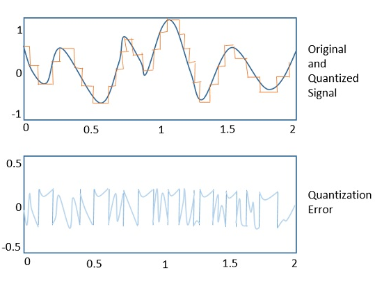
While this error is deterministically linked to the input signal, for many common signals (especially complex ones like speech or music), the error sequence $e[n]$ appears highly random and unpredictable. This observation motivates modeling the quantization error as a random process, often referred to as quantization noise.

The Four Key Assumptions

To build a tractable model, we rely on a set of standard assumptions about the quantization noise $e[n]$. Your background in random processes will be helpful here.

To summarize, the standard model for quantization noise assumes that the error sequence $e[n]$ has the following properties:

1. Stationarity: The statistical properties of the error (like its mean and variance) do not change over time.
2. Uniform Distribution: For rounding to the nearest level, the error is equally likely to be any value within the range from $-\Delta /2$ to $+\Delta /2$, where $\Delta$ is the quantization step size (also known as the LSB). This gives a uniform probability density function (PDF), $p(e)=1/\Delta$ for $e\in [-\Delta /2,\Delta /2]$, and 0 otherwise.
3. Uncorrelation (White Noise): The value of the error at any time sample, $e[n]$, is uncorrelated with the error at any other time sample, $e[m]$, for $n\ne m$. This implies that the noise has a flat power spectral density.
4. Signal Independence: The error sequence $e[n]$ is uncorrelated with the original signal sequence $x[n]$.

As the video notes, these assumptions are most valid when the quantization step $\Delta$ is small and the signal is "busy" enough to cross several quantization levels between samples. For very simple, periodic signals that are harmonically related to the sampling rate, the error can become correlated with the signal, but for most practical applications, this additive white noise model is remarkably effective.

2. Quantifying the Noise: Power and SNR

With a statistical model in hand, we can now calculate the power of the quantization noise. In signal processing, the average power of a zero-mean random process is equal to its variance, ${\sigma }_e^2=E[e^2]$.

Deriving the Noise Power

Given the uniform distribution of the error, we can calculate its variance by integrating $e^2$ against its PDF.

As derived in the video, the calculation is as follows:
${\sigma }_e^2=E[e^2]={\int }_{-\infty }^{\infty }{e}^{2}p(e)de={\int }_{-\Delta /2}^{\Delta /2}{e}^2\frac{1}{\Delta }de$
${\sigma }_e^2=\frac{1}{\Delta }{\left[\frac{e^3}{3}\right]}_{-\Delta /2}^{\Delta /2}=\frac{1}{3\Delta }\left[{\left(\frac{\Delta }{2}\right)}^3-{\left(-\frac{\Delta }{2}\right)}^3\right]=\frac{1}{3\Delta }\left[\frac{{\Delta }^3}{8}+\frac{{\Delta }^3}{8}\right]=\frac{1}{3\Delta }\frac{2{\Delta }^3}{8}$
${\sigma }_e^2=\frac{{\Delta }^2}{12}$

This is a cornerstone result: The average power of quantization noise is ${\Delta }^2/12$. This holds for any signal, provided our initial modeling assumptions are met.

Deriving the Signal-to-Quantization-Noise Ratio (SQNR)

The impact of noise is best understood relative to the signal's strength. The Signal-to-Quantization-Noise Ratio (SQNR) is the ratio of signal power (${\sigma }_x^2$) to noise power (${\sigma }_e^2$).

$SQNR=\frac{{\sigma }_x^2}{{\sigma }_e^2}=\frac{{\sigma }_x^2}{{\Delta }^2/12}$

This formula is general, but to get the famous 6.02N + 1.76 dB result, we need to make an assumption about the input signal. A standard benchmark is a full-scale sine wave.

Let's walk through the key steps from the Analog Devices note and the Van Veen video:

1. Relate $\Delta$ to the number of bits, N: For an ADC with $N$ bits covering a full-scale peak-to-peak range of $V_{pp}$, the step size is $\Delta =V_{pp}/2^N$.
2. Calculate Signal Power ${\sigma }_x^2$: For a full-scale sine wave, the amplitude is $A=V_{pp}/2$. The power (mean-square value) of a sinusoid with amplitude A is $A^2/2$.
   ${\sigma }_x^2=\frac{(V_{pp}/2{)}^2}{2}=\frac{V_{pp}^2}{8}$
3. Combine the terms:
   $SQNR=\frac{{\sigma }_x^2}{{\sigma }_e^2}=\frac{V_{pp}^2/8}{{\Delta }^2/12}=\frac{V_{pp}^2/8}{(V_{pp}/2^N{)}^2/12}=\frac{V_{pp}^2/8}{V_{pp}^2/(12\cdot 2^{2N})}=\frac{12\cdot 2^{2N}}{8}=1.5\cdot 2^{2N}$
4. Convert to Decibels (dB):
   $SQN{R}_{dB}=10{\log }_{10}(1.5\cdot 2^{2N})=10{\log }_{10}(1.5)+10{\log }_{10}(2^{2N})$
   $SQN{R}_{dB}=1.76+20N{\log }_{10}(2)$
   Since $20{\log }_{10}(2)\approx 6.02$, we arrive at the final formula:
   $SQN{R}_{dB}\approx 6.02N+1.76\text{dB}$

This equation is a fundamental result in digital signal processing. It precisely quantifies the trade-off between the number of bits used to represent a signal and the best-case signal-to-noise ratio you can achieve. The 6.02N term is the mathematical origin of the "6 dB per bit" rule of thumb. The 1.76 dB term is a constant that arises specifically from assuming a sinusoidal test signal.

3. System-Level Impact

It is crucial to remember where this noise gets injected. In the case of an ADC, the quantization noise is added to the signal before any digital processing.

This means that if you apply a digital filter to the quantized signal, you are filtering the noise as well. The filter's frequency response will shape the noise spectrum. For example, if you apply a narrow bandpass filter, you will filter out most of the broadband quantization noise, effectively increasing the SNR within that band. This concept, known as "process gain," is a key principle in oversampling converters and software-defined radio, topics we may touch on later.

Conclusion

In this lesson, we put a rigorous mathematical framework around the concept of quantization error. By modeling it as an additive random process, we were able to quantify its impact and derive one of the most important formulas in DSP.

Key Takeaways:

• Quantization error is commonly modeled as an additive, stationary, white noise process that is uniformly distributed between $-\Delta /2$ and $+\Delta /2$.
• The average power of this quantization noise is ${\sigma }_e^2={\Delta }^2/12$, where $\Delta$ is the step size.
• For an N-bit quantizer with a full-scale sinusoidal input, the theoretical maximum Signal-to-Quantization-Noise Ratio is given by $SQN{R}_{dB}\approx 6.02N+1.76\text{dB}$.
• This derivation provides the formal justification for the "6 dB per bit" rule, showing that each additional bit of resolution increases the theoretical SNR by approximately 6 dB.

Preview of the Next Lesson:

We have now deeply analyzed the sources and effects of finite precision. In the next lesson, we will shift gears to another advanced and powerful area of DSP: multirate signal processing. We will explore the fundamental operations of decimation (downsampling) and interpolation (upsampling), learning how to efficiently change the sampling rate of a signal in the digital domain. This is a critical technique used in fields ranging from digital audio to modern telecommunications systems.