Simple Linear Regression with scikit-learn

1. The Core Idea: Modeling a Linear Relationship

Simple linear regression is used when we want to model the relationship between two continuous variables. We assume that this relationship can be approximated by a straight line.

• The independent variable (or feature), denoted as $X$, is the variable we use to make a prediction.
• The dependent variable (or target), denoted as $Y$, is the variable we want to predict.

The relationship is captured by a simple equation that should be familiar from algebra:

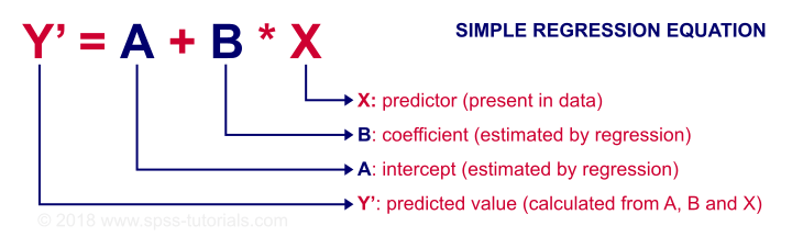
In this equation:

• A (the intercept) is the value of $Y$ when $X$ is 0. It's the point where the line crosses the vertical axis.
• B (the coefficient or slope) represents the change in $Y$ for a one-unit increase in $X$. It tells us how steep the line is and in what direction (positive or negative).

The goal of "training" a linear regression model is to find the best possible values for the intercept (A) and the coefficient (B) that create a line that best fits our data. "Best fit" means the line that minimizes the total distance between itself and the actual data points. This distance is called the error or residual.

To solidify your understanding of these core terms, please read the following brief article section.

2. Fitting a Model with Scikit-Learn: A Practical Example

Now, let's move from theory to practice. We will build a model to predict house prices based on their area in square feet. This is a classic simple linear regression problem: we have one feature (area) to predict one target (price).

The following video from the codebasics YouTube channel provides an excellent, step-by-step walkthrough. We'll watch it in segments to focus on each part of the process.

First, let's see how the problem is set up and how the data is loaded and visualized.

With the data loaded, the next step is to create a LinearRegression object and train it on our data using the .fit() method. This single method call is where scikit-learn performs the "least squares" calculation to find the optimal intercept and coefficient for our best-fit line.

A crucial detail in the video is the use of df[['area']] (with double brackets) as the first argument to .fit(). Scikit-learn's models expect the input features X to be a 2D array-like structure (like a pandas DataFrame or a NumPy array with 2 dimensions), even if you only have one feature. The target y is expected to be a 1D structure (like a pandas Series). This is a common point of confusion for beginners, so it's important to remember!

3. Interpreting the Model's Coefficients

Our model is now trained! But what did it learn? We can inspect the intercept_ and coef_ attributes to find the parameters of our best-fit line. This is the heart of model interpretation.

Let's see how to access these values and, more importantly, understand what they mean in the context of our housing price data.

Let's break down the interpretation shown in the video:

• reg.intercept_: This gives us the intercept ($b$). In our example, it's approximately 180616. Theoretically, this is the predicted price of a house with an area of 0 square feet. While a 0-sq-ft house doesn't make practical sense, the intercept is a necessary part of the equation that anchors the line.
• reg.coef_: This gives us the coefficient ($m$). In our example, it's approximately 135.78. This is the most interpretable part of the model. It means that for every one square foot increase in a home's area, our model predicts the price will increase by approximately $135.78.

This ability to translate a model's coefficient into a simple, real-world statement is a key skill in data science.

4. Visualizing the Model

A great way to confirm our model has learned a reasonable relationship is to visualize it. We can create a scatter plot of our original data and then overlay the regression line that our model has learned.

The resulting plot shows the line cutting through the data points, visually representing the linear trend the model captured. This is a powerful and intuitive way to see your model in action.

Conclusion

Congratulations! You've successfully trained your first supervised learning model. You took a real-world dataset, used scikit-learn to fit a simple linear regression model, and, most importantly, interpreted its coefficients to understand the relationship it discovered.

Key Takeaways:

• Simple linear regression models the relationship between one independent variable ($X$) and one dependent variable ($Y$) using the equation $Y=b+mX$.
• The intercept ($b$) is the predicted value of $Y$ when $X=0$.
• The coefficient ($m$) is the predicted change in $Y$ for a one-unit increase in $X$.
• In scikit-learn, you instantiate LinearRegression(), train it with .fit(X, y), and access the parameters via .intercept_ and .coef_.
• You use the trained model to make predictions with the .predict(X_new) method.

Preview of the next lesson:

We've built a model, but how good is it? Is a predicted price increase of $135.78 per square foot accurate? To answer these questions, we need to evaluate our model's performance quantitatively. In the next lesson, you will learn to evaluate a regression model using key metrics: MSE, RMSE, MAE, and R-squared. This will allow you to move beyond just fitting a model to rigorously assessing its accuracy.