Simple Imputation for Missing Data

1. The Problem of Missing Data

Before we can fix a problem, we need to understand it. In data science, you'll frequently encounter datasets with missing information, often represented as NaN (Not a Number), None, or some other placeholder.

Why do we need to handle them? As mentioned, most algorithms in libraries like scikit-learn will simply fail if they encounter missing values. So, we have two primary options: get rid of the data with missing values, or fill them in.

Let's read a brief overview of these strategies.

As the article points out, while deleting rows or columns (dropna()) is easy, it's often a poor choice because you can lose a significant amount of valuable data. A much more common approach is imputation, which means filling in the missing entries with an estimated or calculated value.

2. Choosing Your Imputation Strategy

The core of this lesson is learning which value to fill in. For simple imputation, we rely on the statistical properties of the column where the data is missing. The three most common strategies are:

• Mean Imputation: Replacing missing values with the average of the column.
• Median Imputation: Replacing missing values with the median of the column.
• Mode Imputation: Replacing missing values with the most frequent value (the mode) of the column.

The choice is not random; it depends on the data's characteristics, which you already know how to investigate from our EDA module!

Let's explore the pros and cons of each method.

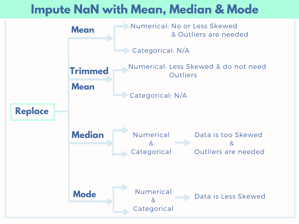
Here's a quick summary of the decision process:

• For numerical data:
  • If the data distribution is symmetrical (like a normal distribution), the mean is a good choice.
  • If the data is skewed or has significant outliers, the median is a much safer, more robust choice because it isn't affected by extreme values.
• For categorical data:
  • The concepts of mean and median don't apply. The only sensible choice is the mode (i.e., the most frequent category).

This diagram visually demonstrates how the mean, median, and mode are positioned in different data distributions. You can see how in a skewed distribution, the mean is "pulled" by the long tail, making it less representative of the central tendency compared to the median.

To make this even more practical, here is a flowchart that can guide your decision-making when you encounter a column with missing values.

3. Practical Imputation with Scikit-learn

Now that we understand the "why" and "what," let's focus on the "how." While you can perform these calculations using pandas (e.g., df['column'].fillna(df['column'].mean())), the standard and most scalable approach in a machine learning project is to use scikit-learn's SimpleImputer. It's designed to fit neatly into a larger ML pipeline, a concept we'll build on throughout this course.

This video provides a concise, practical demonstration of how to use SimpleImputer.

To summarize the process shown in the video, here's the typical workflow in Python:

1. Import necessary libraries.
2. Create an instance of SimpleImputer, specifying your chosen strategy.
3. Fit the imputer to your data to learn the statistic (e.g., the mean).
4. Transform your data to fill in the missing values.

Here's a self-contained code snippet demonstrating this on a small DataFrame with both numerical and categorical features:

import pandas as pd
import numpy as np
from sklearn.impute import SimpleImputer




# 1. Sample data with missing values
data = {'Age': [25, 30, np.nan, 35, 40],
        'City': ['New York', 'London', 'Paris', 'Tokyo', np.nan]}
df = pd.DataFrame(data)
print("Original DataFrame:")
print(df)
print("\nMissing values count:")
print(df.isnull().sum())




# 2. Impute the numerical 'Age' column with the median
# We reshape with .values.reshape(-1, 1) because the imputer expects a 2D array
median_imputer = SimpleImputer(strategy='median')
df['Age'] = median_imputer.fit_transform(df[['Age']])




# 3. Impute the categorical 'City' column with the mode
mode_imputer = SimpleImputer(strategy='most_frequent')
df['City'] = mode_imputer.fit_transform(df[['City']])

print("\nDataFrame after imputation:")
print(df)
print("\nMissing values count after imputation:")
print(df.isnull().sum())

A Crucial Concept: Avoiding Data Leakage

When you start building models, you will split your data into a training set and a testing set. It is critical that you only fit your imputer on the training data. You learn the mean, median, or mode from the training data and then use that learned statistic to transform both the training and the test data.

Why? Fitting on the entire dataset before splitting would mean you are using information from the test set to process your training set. This "leaks" information from the future (the test set) into your training process, leading to an overly optimistic evaluation of your model's performance.

We will put this into practice in a later module, but it's a vital concept to understand now. The fit_transform() shortcut we used above is only safe to use on your training data.

Conclusion

Great work! You've just learned one of the most common and essential data preprocessing tasks. Handling missing data is a necessary chore that makes machine learning possible on real-world, imperfect datasets.

Key Takeaways:

• Most machine learning models require complete data, so handling missing values is a mandatory preprocessing step.
• Simple imputation involves replacing missing values with a statistic: mean, median, or mode.
• The choice of strategy depends on the data:
  • Median is robust for skewed numerical data or data with outliers.
  • Mean works well for symmetrical numerical data.
  • Mode is the standard choice for categorical data.
• Scikit-learn's SimpleImputer is the standard tool for this task, and it's crucial to fit it only on training data to prevent data leakage.

Preview of the next lesson:

We've successfully filled in the gaps in our data. But what about the 'City' column? Even though it has no missing values now, a machine learning model can't understand text like 'New York' or 'London'. In our next lesson, we will tackle this by learning how to encode categorical variables, turning them into the numbers that models require.