Explained Variance in PCA

1. The Core Idea: What is "Explained Variance"?

In the last lesson, we established that PCA finds new axes (principal components) that capture the maximum amount of "spread" or variance in the data. The first principal component (PC1) captures the most, PC2 captures the second most, and so on.

Explained variance is simply the percentage of the total variance in the original dataset that is captured by each principal component.

If PC1 has an explained variance of 70%, it means that this single new feature captures 70% of the information about the spread of our data. If we add PC2, which explains 20%, then together our two new features capture 90% of the total variance.

To build a solid intuition for this, let's return to the excellent StatQuest series.

As the video explains, the variance captured by each principal component is quantified by a value called its eigenvalue ($\lambda$). The larger the eigenvalue, the more variance the component explains.

Therefore, the explained variance ratio for a specific component $i$ is calculated by dividing its eigenvalue by the sum of all eigenvalues:

Where $N$ is the total number of components (which is equal to the original number of features).

This formula is the mathematical heart of what we mean by "explained variance". Let's get another perspective on this that connects it more formally to the underlying linear algebra.

2. Visualizing and Interpreting Explained Variance

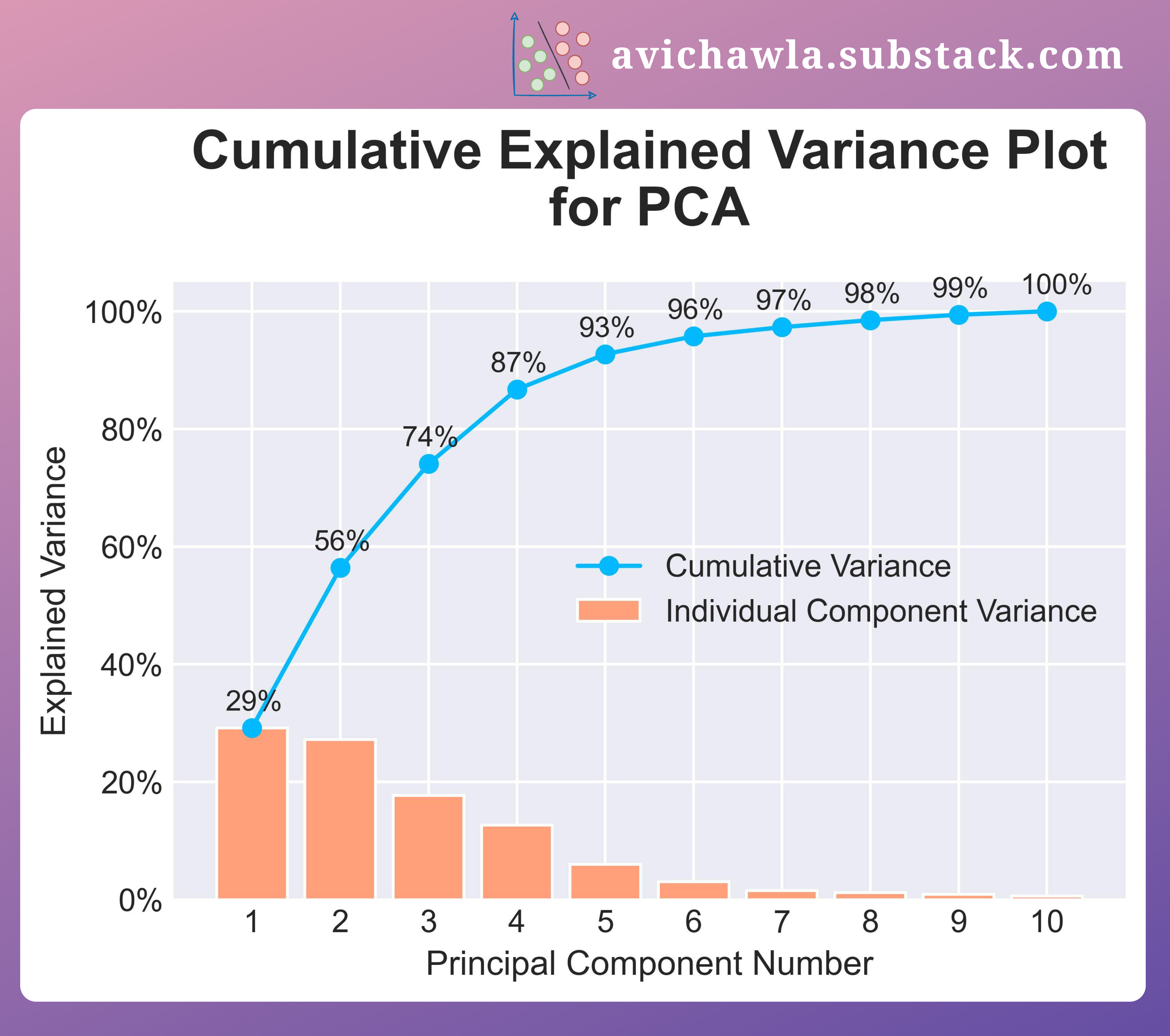
Knowing the formula is one thing; using it is another. In practice, we rarely calculate this by hand. Instead, we use visualizations to help us decide how many components to keep. The two most common plots are the Scree Plot and the Cumulative Explained Variance Plot.

• Scree Plot: A bar chart showing the explained variance for each individual principal component, sorted in descending order. It helps you see the point of "diminishing returns," where adding more components doesn't add much new information.
• Cumulative Explained Variance Plot: A line plot showing the total variance explained as you add components one by one. This plot directly answers the question, "How many components do I need to capture X% of the variance?"

The following article provides a great hands-on guide to creating and interpreting these plots.

To make this even more concrete, here is an example of a plot that combines both visualizations.

3. Making the Decision: How Many Components to Keep?

You now have the tools to make an informed decision. The number of components you choose is a trade-off.

• Too few components: You risk losing important information, potentially hurting the performance of any subsequent machine learning model.
• Too many components: You retain most of the information but gain little in terms of dimensionality reduction, defeating the purpose of PCA.

Here are two common strategies for choosing the optimal number:

1. The Threshold Method:
This is what we implicitly did in the last lesson. You set a threshold (e.g., 95%) and keep the smallest number of components required to meet it. This is the most common approach when PCA is used for preprocessing before feeding data into another model. The cumulative explained variance plot is your best tool here.

The following article shows the code for implementing this logic.

2. The Elbow Method (using the Scree Plot):
You look at the scree plot and find the "elbow"—the point where the explained variance of subsequent components drops off and the curve flattens. The components before the elbow are considered the most significant ones to retain. This method is more of a heuristic but is very useful for getting a quick sense of the data's intrinsic dimensionality.

Let's see one final example of how this is applied when deciding whether a 2D plot is a good representation of a high-dimensional dataset.

Conclusion

Excellent work! You've now unpacked one of the most important concepts in PCA. Understanding explained variance moves you from being a user of a black-box algorithm to an informed practitioner who can diagnose and justify your modeling choices.

Key Takeaways:

• Explained variance is the proportion of a dataset's total variance that is captured by a principal component.
• It is calculated from the eigenvalues associated with each component. In scikit-learn, this is accessible via the .explained_variance_ratio_ attribute after fitting a PCA model.
• We use a Scree Plot to see the variance of individual components and a Cumulative Explained Variance Plot to see the total variance captured as we add more components.
• These plots allow us to make an informed decision about the number of components to keep, either by setting a variance threshold (e.g., 95%) or finding the "elbow" in the scree plot.

Preview of the next lesson:
In this lesson, we confirmed that checking the explained variance is crucial before deciding to visualize data in a lower dimension. In our next lesson, we will put this into practice and focus on the final step: visualizing high-dimensional data in two dimensions using PCA. We will apply what we've learned to create, interpret, and label these powerful visualizations.