Fixed-Size Hash Tables: Linear Probing & Tombstone Deletions

1. Hash Table Fundamentals

A hash table is a data structure that maps keys to values for highly efficient lookup. In the ideal case, it can find any element in constant time, or O(1), regardless of how many items are in the table. This is a significant advantage over the O(log n) of balanced trees or the O(n) of linked lists.

The core components are:

• An array of "buckets" where data is stored.
• A hash function that converts a given key into an index in the array.

The main challenge with hash tables is handling collisions. Since the number of possible keys is usually much larger than the number of buckets in our array, multiple keys will inevitably map to the same index. The strategy used to resolve these collisions is what defines the hash table's performance and complexity.

2. Open Addressing and Linear Probing

There are two primary strategies for collision resolution:

1. Separate Chaining: Each bucket stores a pointer to a linked list of all key-value pairs that hash to that index. This requires dynamic memory allocation for list nodes, which is often undesirable in embedded systems.
2. Open Addressing: All key-value pairs are stored directly in the bucket array. When a collision occurs, we "probe" or search for the next available bucket according to a set sequence.

For this lesson, we will focus on linear probing, the simplest form of open addressing. If a bucket is occupied, we simply check the next one in the array, and the next, and so on, wrapping around to the beginning if necessary, until we find an empty slot.

While simple and cache-friendly, linear probing can lead to primary clustering, where long runs of occupied buckets form, degrading lookup performance to O(n) in the worst case.

3. The Deletion Problem: Breaking the Chain

Now for the critical interview question: what happens when you delete an element from a hash table that uses linear probing?

If we simply find the element and clear its bucket, we can break the probe sequence. Any elements that collided with that slot and were placed after it will become unreachable.

4. The Solution: Tombstones

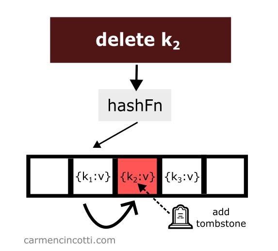
To solve this, we introduce a third state for our buckets. A bucket is no longer just "occupied" or "empty"; it can also be "deleted". We mark a deleted slot with a special value called a tombstone.

This changes the rules for our operations:

• Lookup: The probe sequence continues past tombstones. It only stops when it finds the target key or an empty (never-used) bucket.
• Insert: Can place the new element in the first empty bucket or the first tombstone it encounters. Reusing tombstone slots is an important optimization.
• Delete: Finds the element and replaces its bucket with a tombstone.

5. Implementation in C

Let's implement a fixed-size hash table that embodies these principles. We will create a robust implementation suitable for an embedded system, using a fixed-size array and an enum to manage bucket state.

5.1 Data Structures

First, we define the states, the key-value entry, and the hash table itself.

#include <stdio.h>
#include <stdlib.h>
#include <string.h>
#include <stdbool.h>




#define TABLE_SIZE 16 // A fixed size for our embedded context

typedef enum {
    EMPTY,
    OCCUPIED,
    DELETED
} EntryState;

typedef struct {
    const char* key;
    int value;
    EntryState state;
} HashEntry;

typedef struct {
    HashEntry entries[TABLE_SIZE];
} HashTable;

// A simple hash function (djb2)
unsigned long hash_function(const char *str) {
    unsigned long hash = 5381;
    int c;
    while ((c = *str++)) {
        hash = ((hash << 5) + hash) + c; /* hash * 33 + c */
    }
    return hash;
}

void ht_init(HashTable* table) {
    for (int i = 0; i < TABLE_SIZE; i++) {
        table->entries[i].key = NULL;
        table->entries[i].value = 0;
        table->entries[i].state = EMPTY;
    }
}

5.2 The Core Logic: ht_find_entry

The most complex logic is encapsulated in a helper function that finds the correct bucket for a given key. This function needs to correctly handle all three bucket states.

// Internal helper to find a bucket for a key.
// Returns a pointer to the bucket where the key is, or where it should be inserted.
static HashEntry* ht_find_entry(HashEntry* entries, const char* key) {
    unsigned long index = hash_function(key) % TABLE_SIZE;
    HashEntry* tombstone = NULL;

    for (int i = 0; i < TABLE_SIZE; i++) {
        // Calculate the probing index
        unsigned long probe_index = (index + i) % TABLE_SIZE;
        HashEntry* entry = &entries[probe_index];

        switch (entry->state) {
            case EMPTY:
                // If we found an empty slot, the key isn't here.
                // If we passed a tombstone, return it for reuse. Otherwise, return this empty slot.
                return tombstone != NULL ? tombstone : entry;

            case DELETED:
                // Found a tombstone. We can insert here, but we must keep searching
                // to see if the key already exists further down the probe chain.
                if (tombstone == NULL) {
                    tombstone = entry;
                }
                break;

            case OCCUPIED:
                // If keys match, we found it.
                if (strcmp(entry->key, key) == 0) {
                    return entry;
                }
                break;
        }
    }
    
    // This should ideally not be reached if the table is not full.
    // In a real system you'd handle this table-full error.
    return tombstone; 
}

This logic is subtle but crucial. Notice how it prioritizes finding an existing key over reusing a tombstone, but remembers the first tombstone encountered in case the key isn't found and an insertion is intended.

5.3 Public API: Insert, Lookup, Delete

With ht_find_entry, the public functions become much cleaner.

// Insert or update a key-value pair. Returns true on success.
bool ht_insert(HashTable* table, const char* key, int value) {
    HashEntry* entry = ht_find_entry(table->entries, key);
    if (entry == NULL) {
        // Table is full of occupied slots (no empty or tombstone slots available)
        return false;
    }

    bool is_new_key = (entry->state != OCCUPIED);
    
    entry->key = key;
    entry->value = value;
    entry->state = OCCUPIED;

    return is_new_key;
}

// Look up a key. Returns true and sets 'value' if found.
bool ht_lookup(HashTable* table, const char* key, int* value) {
    HashEntry* entry = ht_find_entry(table->entries, key);
    if (entry == NULL || entry->state != OCCUPIED) {
        return false;
    }
    *value = entry->value;
    return true;
}

// Delete a key. Returns true if the key was found and deleted.
bool ht_delete(HashTable* table, const char* key) {
    HashEntry* entry = ht_find_entry(table->entries, key);
    if (entry == NULL || entry->state != OCCUPIED) {
        // Key not found
        return false;
    }

    // Place the tombstone
    entry->state = DELETED;
    entry->key = NULL; // Optional: clear dangling pointers
    entry->value = 0;

    return true;
}

6. Interview Discussion: The Downsides of Tombstones

Simply knowing how to implement tombstones is good; being able to discuss their trade-offs is what distinguishes a senior candidate.

Key Discussion Points:

1. Performance Degradation: The biggest issue is that tombstones fill up the table. A table can be "full" of tombstones, making searches for non-existent keys an O(n) operation because the probe must traverse all the tombstones before finding an EMPTY slot.
2. Memory Overhead: While we don't store extra data per se, a tombstone occupies a slot that could be used for new data, effectively increasing the logical load factor and collision rate over time if many deletions occur.
3. Cleanup/Rehashing: To combat performance degradation, a system might periodically perform a rehash: create a new, empty hash table and insert all the OCCUPIED items from the old table into the new one. This expensive operation cleans out all tombstones. In an embedded system, this might happen during a designated maintenance period or idle task.

Deeper Dive: An Alternative to Tombstones

For extra credit in an interview, you can mention an alternative called backward-shift deletion.

• When an item is deleted, you iterate forward through the probe chain.
• For each subsequent item, you check if it can be "shifted back" one spot (into the now-empty slot) without breaking its own probe chain.
• This is repeated until you hit an empty bucket.

This keeps the probe chains compact and avoids tombstones entirely, but makes the delete operation much more expensive. The choice between tombstones (fast delete, slower lookup over time) and backward-shifting (slow delete, fast lookup) is a classic engineering trade-off.

Conclusion

You have successfully designed and implemented a fixed-size hash table with linear probing, a staple of coding interviews. You've tackled the non-trivial deletion problem by implementing tombstones and, more importantly, you can now discuss the performance implications and alternatives like a senior engineer.

Key Takeaways:

• Open addressing with linear probing stores all entries in the main array, which is cache-friendly but prone to clustering.
• Naively deleting an entry breaks the probe chain, making subsequent elements unreachable.
• Tombstones solve this by marking deleted slots, creating three states: EMPTY, OCCUPIED, and DELETED.
• insert and lookup operations must be modified to handle tombstones: insert can reuse them, while lookup must probe past them.
• The main drawback of tombstones is performance degradation over time, which may necessitate a full table rehash to clean them out.

Preview of the Next Lesson:

We've covered two essential data structures: heaps for prioritization and hash tables for lookups. We will now move to a lower level of data manipulation that is critical in embedded programming: fixed-point arithmetic. In the next lesson, you will learn to explain fixed-point representation (Q notation) and implement basic arithmetic operations, a skill essential for doing math on processors without a floating-point unit (FPU).