Single-Pass Variance Formula Derivation

Hello! Welcome to your course on Welford's algorithm.

Your goal is to understand the theory, derivation, and implementation of this powerful algorithm. Given your background in data science and machine learning, you know that calculating statistics like mean and variance is a fundamental task. However, the standard methods can sometimes fail in surprising ways on a computer.

This course is structured to build your understanding from the ground up. We'll start by exploring the challenges of calculating variance, which will reveal why a specialized algorithm like Welford's is necessary. Then, we will dive into the derivation and implementation of Welford's algorithm itself.

In this first lesson, we will focus on a foundational piece of the puzzle. Our goal is to derive the common single-pass 'textbook' formula for variance from its statistical definition. This will lay the groundwork for understanding both the potential efficiencies and the hidden dangers of variance calculation.

1. Defining Mean and Variance

Let's start with a quick refresher on the fundamental definitions of mean and variance. For a dataset with $N$ data points ${x_{1}, x_{2}, \dots, x_{N}}$ , the mean ( $μ$ ) is simply the average of all the data points:

$μ = \frac{1}{N} \sum_{i = 1}^{N} x_{i}$

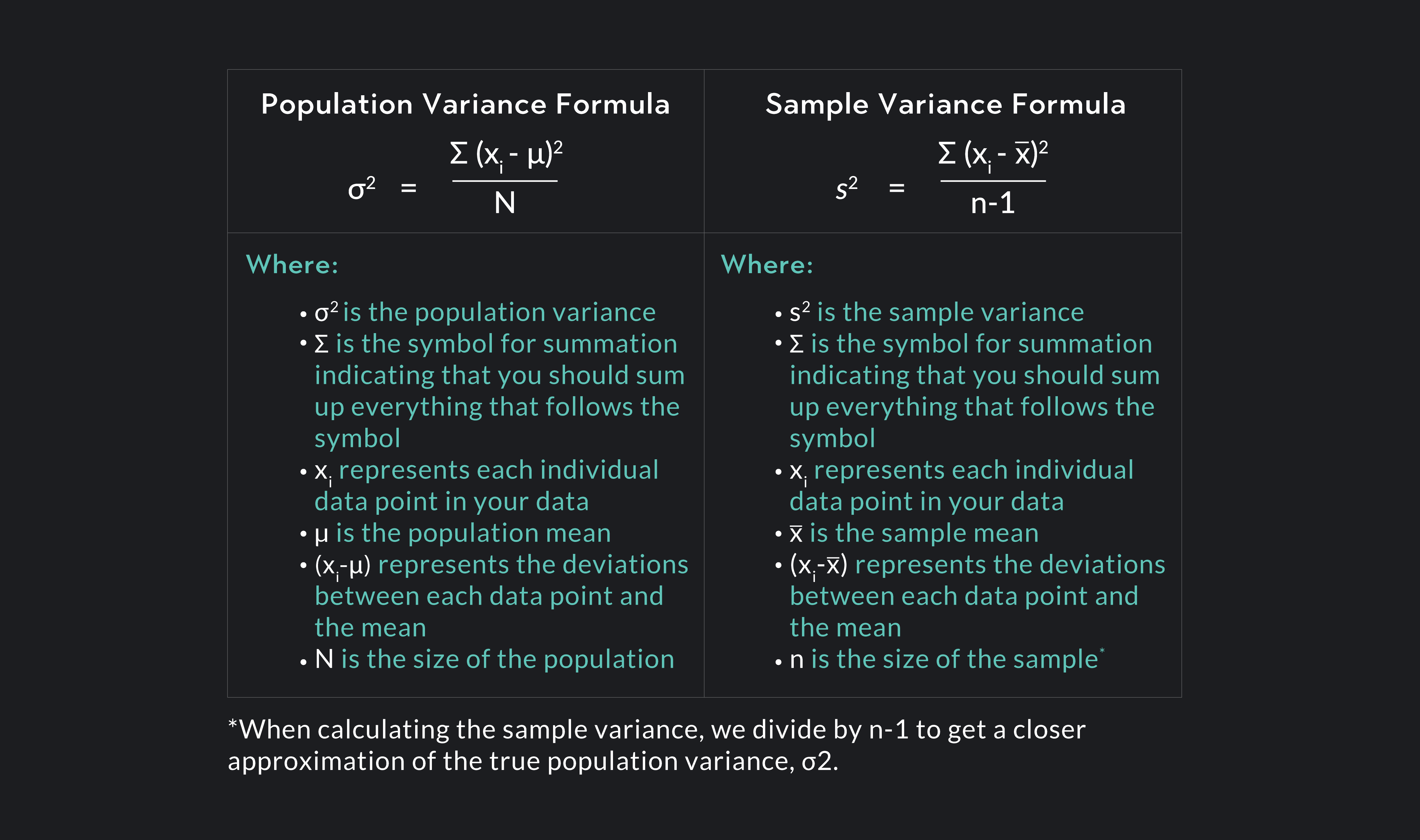
The variance ( $σ^{2}$ ) measures the average squared deviation of each data point from the mean. It tells us how "spread out" the data is. Its definitional formula is:

$σ^{2} = \frac{1}{N} \sum_{i = 1}^{N} (x_{i} - μ)^{2}$

The image below distinguishes between population variance (when you have data for an entire population) and sample variance (when you have a sample from a larger population).

Population vs. Sample Variance Formulas — This image shows the formulas for population variance (using $N$ in the denominator) and sample variance (using $n-1$). For our derivations, we will use the population variance formula, but the same algebraic principles apply to both.

The definitional formula is intuitive, but implementing it directly requires two passes over the data:

First pass: Calculate the mean ( $μ$ ).
Second pass: Use the calculated mean to find the sum of squared differences, $\sum (x_{i} - μ)^{2}$ .

This can be inefficient for large datasets that don't fit into memory. This motivates us to find a formula that can be computed in a single pass.

2. Deriving the Single-Pass "Shortcut" Formula

We can algebraically rearrange the definitional formula for variance into a more computationally convenient form. This new form is often called the "shortcut" or "textbook" formula.

To see how this is done, I recommend you read through a formal derivation. The following resource from ProbabilityCourse.com provides a clear, step-by-step proof.

Variance | Standard Deviation

This reading from ProbabilityCourse.com walks through the mathematical proof for the computational formula for variance. It uses the language of expected values, which provides a solid theoretical foundation that aligns well with your background in math and machine learning.

Please read the section titled 'Computational formula for the variance'. Focus on how the linearity of expectation is used to rearrange the terms. The proof starts with Var(X) = E[(X - μ_X)^2] and ends with Var(X) = E[X^2] - [EX]^2.

Let's walk through that derivation again, using the summation notation for a finite dataset. This will make the connection to computation more direct.

Start with the definition of variance:
$σ^{2} = \frac{1}{N} \sum_{i = 1}^{N} (x_{i} - μ)^{2}$
Expand the squared term inside the summation: $(x_{i} - μ)^{2} = x_{i}^{2} - 2 x_{i} μ + μ^{2}$ .
$σ^{2} = \frac{1}{N} \sum_{i = 1}^{N} (x_{i}^{2} - 2 x_{i} μ + μ^{2})$
Distribute the summation across the three terms:
$σ^{2} = \frac{1}{N} (\sum_{i = 1}^{N} x_{i}^{2} - \sum_{i = 1}^{N} 2 x_{i} μ + \sum_{i = 1}^{N} μ^{2})$
Factor out constants from the summations. Remember that $μ$ is a constant for the entire dataset. The term $2 μ$ can be pulled out of the second summation, and $μ^{2}$ can be pulled out of the third.
$σ^{2} = \frac{1}{N} (\sum x_{i}^{2} - 2 μ \sum x_{i} + \sum μ^{2})$
Note that summing the constant $μ^{2}$ for $N$ times is simply $N μ^{2}$ .
$σ^{2} = \frac{1}{N} (\sum x_{i}^{2} - 2 μ \sum x_{i} + N μ^{2})$
Substitute the definition of the mean. We know that $μ = \frac{1}{N} \sum x_{i}$ . This can be rewritten as $\sum x_{i} = N μ$ . Let's substitute this into the equation:
$σ^{2} = \frac{1}{N} (\sum x_{i}^{2} - 2 μ (N μ) + N μ^{2})$
Simplify the expression:
$σ^{2} = \frac{1}{N} (\sum x_{i}^{2} - 2 N μ^{2} + N μ^{2})$
$σ^{2} = \frac{1}{N} (\sum x_{i}^{2} - N μ^{2})$
$σ^{2} = \frac{\sum x _{i}^{2}}{N} - μ^{2}$

And there we have it! This is the single-pass formula for variance:

$σ^{2} = \frac{\sum x _{i}^{2}}{N} - (\frac{\sum x _{i}}{N})^{2}$

This formula is powerful because it allows us to calculate variance by iterating through the data only once, keeping track of just three quantities:

The number of data points, $N$ .
The sum of the data points, $\sum x_{i}$ .
The sum of the squares of the data points, $\sum x_{i}^{2}$ .

Once we have these three sums, we can compute the mean and variance without needing to store the entire dataset. This is ideal for processing data streams or very large files.

Test your understanding!

Consider the small dataset: ${2, 3, 5, 6}$ .

Calculate the variance using the two-pass definitional formula: $σ^{2} = \frac{1}{N} \sum (x_{i} - μ)^{2}$ .
Calculate the variance using the single-pass formula we just derived: $σ^{2} = \frac{\sum x _{i}^{2}}{N} - μ^{2}$ .
Verify that both formulas give the same result.

Show answer

The dataset is ${2, 3, 5, 6}$ , so $N = 4$ .

1. Using the two-pass definitional formula:

Pass 1: Calculate the mean ( $μ$ )
$μ = \frac{2 + 3 + 5 + 6}{4} = \frac{16}{4} = 4$
Pass 2: Calculate the sum of squared differences
$\sum (x_{i} - μ)^{2} = (2 - 4)^{2} + (3 - 4)^{2} + (5 - 4)^{2} + (6 - 4)^{2}$
$= (- 2)^{2} + (- 1)^{2} + (1)^{2} + (2)^{2}$
$= 4 + 1 + 1 + 4 = 10$
Calculate variance
$σ^{2} = \frac{10}{4} = 2.5$

2. Using the single-pass formula:

Single Pass: Calculate $N$ , $\sum x_{i}$ , and $\sum x_{i}^{2}$
- $N = 4$
- $\sum x_{i} = 2 + 3 + 5 + 6 = 16$
- $\sum x_{i}^{2} = 2^{2} + 3^{2} + 5^{2} + 6^{2} = 4 + 9 + 25 + 36 = 74$
Calculate variance
$μ = \frac{\sum x _{i}}{N} = \frac{16}{4} = 4$
$σ^{2} = \frac{\sum x _{i}^{2}}{N} - μ^{2} = \frac{74}{4} - 4^{2}$
$= 18.5 - 16 = 2.5$

Both formulas correctly yield a variance of 2.5.

Conclusion

In this lesson, we have achieved our first objective. We started from the intuitive, two-pass definition of variance and mathematically derived an equivalent one-pass formula.

Key Takeaways:

The definitional formula for variance, $σ^{2} = \frac{1}{N} \sum (x_{i} - μ)^{2}$ , requires two passes over the data.
Through algebraic manipulation, we derived the single-pass or "shortcut" formula: $σ^{2} = \frac{\sum x _{i}^{2}}{N} - μ^{2}$ .
This formula is computationally efficient as it only requires one pass through the data to gather the necessary sums ( $N$ , $\sum x_{i}$ , and $\sum x_{i}^{2}$ ).

This single-pass formula seems like a clear winner. However, as you'll see in upcoming lessons, its elegance in mathematics hides a significant flaw in practical computation.

Preview of the Next Lesson:

Next, we will formally examine the two-pass algorithm as a stable (though less efficient) baseline. Then, we will introduce the concept of catastrophic cancellation, a key source of error in computer arithmetic. This will set the stage for understanding exactly why the single-pass formula we just derived can fail dramatically, and why algorithms like Welford's are so important.

Recommended resources

1. Defining Mean and Variance

2. Deriving the Single-Pass "Shortcut" Formula

Conclusion