Dynamic Programming: State and Recurrence

The Anatomy of a DP Solution

At its core, a dynamic programming algorithm consists of three components. A formal definition will be helpful before we dive into the process of deriving them.

To summarize, the two key components we'll focus on are:

1. State: A set of parameters that contains the minimum information required to uniquely describe a subproblem. It's the information we must "carry forward" to make future decisions correctly. Anything not included in the state is considered irrelevant for future choices.
2. Recurrence Relation: An equation that defines the solution of a larger problem (a state) in terms of the solutions of smaller, already-solved subproblems (previous states). This relation mathematically captures the principle of optimal substructure.

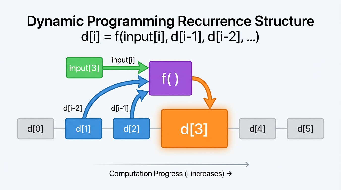
The image below illustrates this structure. The solution for state d[i] is computed by a function f() that takes the current input and the solutions to previous states (d[i-1], d[i-2], etc.) as its arguments. The recurrence is the formal definition of this function f().

The Art of Modeling: An Iterative Process

Defining the state and recurrence for a novel problem is the most creative and challenging part of dynamic programming. It is less a matter of formulaic application and more an engineering process of iterative refinement. Your background in compiler design, where one must choose the right information to store in an Intermediate Representation (IR), is structurally isomorphic to this process. You can't just store the source code verbatim (too much info), nor can you store just the final result (too little info). You need the right abstraction.

The following resource outlines a practical strategy for finding a valid DP model. It frames the process as a form of trial and error.

Let's apply this iterative process to a few examples.

Example 1: Sum Representation

Problem: Given an integer n, in how many ways can it be written as a sum of the integers 1, 3, and 4?

1. Choose an order: A natural order is to solve for n=1, then n=2, n=3, and so on, building up to the target n.
2. Pick a tentative state: Let's define our state dp[i] as "the number of ways to form the sum i". The state is simply the target integer i.
3. Determine the recurrence: To form a sum i, the very last number we added must have been a 1, a 3, or a 4.
   • If the last number was 1, all previous numbers must sum to i-1. The number of ways this could have happened is dp[i-1].
   • If the last number was 3, the previous sum was i-3. The number of ways is dp[i-3].
   • If the last number was 4, the previous sum was i-4. The number of ways is dp[i-4].
     Since these three cases are mutually exclusive, the total number of ways to form i is the sum of the ways from these preceding states.
   $$dp[i]=dp[i-1]+dp[i-3]+dp[i-4]$$ Our tentative state was sufficient. We can express the solution for i using only solutions for smaller values.
4. Identify Base Cases: We need values for the smallest subproblems that don't depend on others. dp[0] = 1 (the empty sum is the one way to make 0). We also need dp[1], dp[2], and dp[3] to get the recurrence started. These can be calculated by hand: dp[1]=1 (1), dp[2]=1 (1+1), dp[3]=2 (1+1+1, 3).

This example is detailed in both of the following resources. You can quickly review them to see the logic in action.

Example 2: The State Refinement Loop

The previous example was straightforward. More often, your first guess at a state will be insufficient, forcing a refinement.

Problem: Given a tree with weights on its vertices, find the maximum weight of an independent set (a subset of vertices where no two are adjacent).

1. Choose an order: A natural order for trees is to process from the leaves up to the root. A post-order traversal is a good mental model.
2. Attempt 1: Insufficient State
   • Tentative State: Let dp[u] be the max weight independent set (MWIS) in the subtree rooted at u.
   • Recurrence Check: To calculate dp[u], we consider two choices for vertex u itself:
     1. Don't include u in the set: The MWIS for the subtree is the sum of the MWIS of the subtrees of its children. So, dp[u] = sum(dp[v]) for all children v of u. This part works.
     2. Include u in the set: If we include u, we cannot include any of its direct children v. The total weight would be weight[u] plus the sum of the MWIS from the subtrees of its grandchildren. Our current state dp[v] doesn't provide this! dp[v] is the MWIS for the entire subtree at v, which might or might not include v itself. We don't have enough information to make the choice at u.
3. Attempt 2: Refined State
   • New State: The issue was that for a child's subtree, we needed to know the solution both with and without the child's root. So let's store both.
     • f(u): the MWIS of the subtree at u that includes u.
     • g(u): the MWIS of the subtree at u that does not include u.
   • Recurrence Check:
     • To compute f(u) (we take u), we must add weight[u] and we cannot take its children. Thus, we must take the sum of g(v) for all children v.
       $f(u)=\text{weight}[u]+{\sum }_{v\in \text{children}(u)}g(v)$
     • To compute g(u) (we don't take u), we are free to either take or not take each child v. For each child v, we can choose the better of the two options, which is max(f(v), g(v)).
       $g(u)={\sum }_{v\in \text{children}(u)}\max (f(v),g(v))$
   • This state representation is sufficient. The final answer for the whole tree (rooted at r) would be max(f(r), g(r)).

This process of hitting a wall and refining the state is central to solving DP problems. The following resource walks through this exact thought process.

State as a Function's Arguments

A powerful way to think about state is to first imagine a brute-force recursive solution. The parameters you pass to your recursive function are, by definition, the state of that subproblem. The goal of DP is to identify which of these parameters are essential and which are redundant.

Let's see this with an example from the HackerEarth tutorial on selling wines.

Problem: You have a row of N wines. Each year you must sell either the leftmost or rightmost wine. The profit of selling a wine is price[i] * year. Find the maximum possible profit.

A naive recursive function might be profit(prices, year, begin_index, end_index).

However, the year is redundant. It can always be calculated from the number of wines already sold. The number of wines sold is N - (end_index - begin_index + 1). So, year = (N - (end_index - begin_index + 1)) + 1.

By removing the redundant parameter, we simplify the state.

• State: A tuple (begin, end), representing the subproblem of finding the max profit for the contiguous block of wines from begin to end.
• Recurrence: From state (begin, end), we have two choices. The current year can be computed as described above.
  1. Sell the leftmost wine: profit = price[begin] * year + solve(begin + 1, end)
  2. Sell the rightmost wine: profit = price[end] * year + solve(begin, end - 1)
     The recurrence is the max of these two choices.

The resource below walks through this exact process of starting with a backtrack solution and minimizing the arguments to find the essential state.

This idea also highlights when DP is not applicable. If making a decision requires the entire history of previous choices, and not just a compressed state, then DP fails. The information is not useless and cannot be discarded. The final example in Colin Galen's video, a grid path problem where you must visit each cell exactly once, illustrates this perfectly. The state would need to include a bitmask of all visited cells, which often makes the solution exponential and no better than backtracking.

Tying it all Together: The DAG Model Revisited

Let's connect this back to our primary abstraction: the dependency DAG.

• The State (i, j, ...) defines a single vertex in the graph. The set of all possible states (e.g., all (i, j) where 0 <= i < N and 0 <= j < M) forms the complete set of vertices.
• The Recurrence Relation dp[i] = f(dp[j], dp[k]) defines the directed edges. In this case, there would be edges j -> i and k -> i.
• Base Cases are the vertices with an in-degree of 0. They are the subproblems that can be solved without any recursive dependencies.

Solving a DP problem is equivalent to traversing this implicitly defined graph and computing the value at each vertex, ensuring that a vertex is computed only after all vertices that have edges leading to it have been computed. This is, by definition, a topological sort of the subproblem graph.

Summary

This lesson focused on the pivotal step of translating a problem into a formal DP model. The key takeaways are:

• State and Recurrence are the core: A DP solution is defined by its state representation and the recurrence relation that connects states.
• State is minimal information: The state must capture just enough information to define a subproblem and allow future choices. It is the set of parameters for a subproblem.
• Recurrence defines dependencies: The recurrence relation expresses the solution to one state in terms of previously solved states, mapping directly to the edges of the subproblem DAG.
• Modeling is iterative: Finding the correct state is often a process of trial and error. Start with a simple guess, and if it's insufficient to form a recurrence, add the necessary information and repeat.
• Recursion informs state: A powerful technique is to formulate a brute-force recursive solution. The parameters of your recursive function are your candidate state.

In our next lesson, we will take the state and recurrence we've defined and implement them. We'll start with a top-down approach using recursion and memoization, which is a very direct translation of the recurrence relations we've been formulating today.