Tabulation and Topological Sort for Dynamic Programming

From "Pull" to "Push": The Bottom-Up Paradigm

In the top-down model, the computation is driven by the recursive calls. The bottom-up model inverts this. It's a "push" mechanism where we pre-determine a valid evaluation order and systematically compute the solution for every subproblem, storing them in a table (hence, "tabulation").

The core idea is that if subproblem A depends on subproblems B and C, we must solve B and C before we can solve A. By iterating through the subproblems in an order that respects these dependencies, we guarantee that whenever we need the solution to a smaller problem, it's already computed and waiting in our table.

This evaluation order is precisely a topological ordering of the subproblem dependency graph, where each subproblem is a node and an edge B -> A signifies that A depends on B.

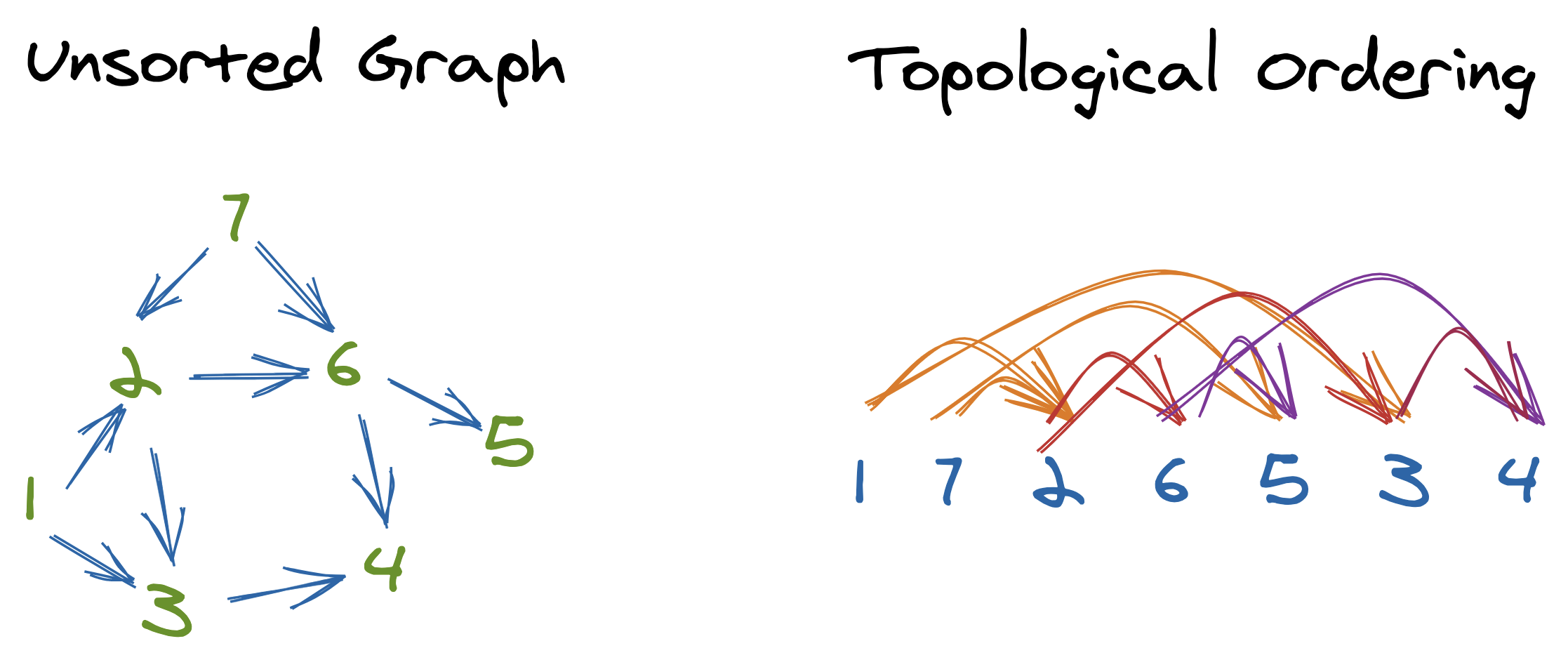
On the left is the dependency graph of subproblems. On the right is a valid topological ordering, which represents a valid evaluation order for a bottom-up DP solution. All dependencies (arrows) point from an earlier position to a later one in the sequence.

The following video provides a clear introduction to this shift in perspective, using the Fibonacci sequence to contrast the top-down memoized strategy with the bottom-up tabulated one. Pay close attention to the explicit connection made between the order of evaluation and the dependencies between subproblems.

As the video highlights, for Fibonacci, the dependency graph is simple: fib(n) depends on fib(n-1) and fib(n-2). A topological sort is simply the natural order of integers 0, 1, 2, ..., n. The bottom-up algorithm hard-codes this trivial topological sort with a simple for loop.

The Isomorphism: DP and DAG Evaluation

This relationship between DP and Directed Acyclic Graphs (DAGs) is not just a useful analogy; it's a structural isomorphism. We can formally state that every dynamic programming problem is equivalent to performing a computation over a DAG of subproblems.

A fantastic set of lecture notes from Jeff Erickson's algorithms course at UIUC solidifies this connection.

The crucial insight here is that you've been working with this pattern all along in compiler design. Evaluating attributes in a syntax tree, scheduling instructions in an intermediate representation, or resolving symbol dependencies—all these are computations on DAGs that require a topological evaluation order. Bottom-up DP is the same principle applied to optimization and counting problems.

Case Study 1: Shortest Paths in a DAG

Let's examine a problem where the dependency graph isn't implicit but is the problem itself: finding the shortest paths from a single source s in a DAG, which may include negative edge weights. Dijkstra's algorithm fails here, but DP provides an elegant and efficient solution.

The following resource from Carnegie Mellon University frames this problem explicitly as a dynamic program evaluated over a DAG.

Let's break this down:

• State: dist(v) is the length of the shortest path from source s to vertex v.
• Recurrence: dist(v) = min_{(u,v) in Edges} { dist(u) + weight(u,v) }
• Base Case: dist(s) = 0, and dist(v) = ∞ for all other v.
• Evaluation Order: A topological sort of the graph's vertices. By processing vertices in this order, we guarantee that when we calculate dist(v), dist(u) for all predecessors u has already been finalized. The algorithm is a direct implementation of bottom-up DP.

Case Study 2: Longest Common Subsequence (LCS)

Now let's apply this to a problem where the DAG is implicit. For the LCS of two strings A and B, the state LCS(i, j) is the length of the LCS for prefixes A[1..i] and B[1..j].

The recurrence is:

The dependency graph here has nodes (i, j) for 0 <= i <= |A| and 0 <= j <= |B|. The recurrence shows that node (i, j) has incoming edges from (i-1, j), (i, j-1), and (i-1, j-1). This forms a grid-like DAG.

What is a valid topological sort? Any path that moves from smaller i, j to larger i, j. The most common "hard-wired" topological sort is to iterate through the DP table row by row, and for each row, column by column.

# A[1..m], B[1..n]
dp = [[0 for _ in range(n + 1)] for _ in range(m + 1)]

for i in range(1, m + 1):
    for j in range(1, n + 1):
        if A[i-1] == B[j-1]:
            dp[i][j] = 1 + dp[i-1][j-1]
        else:
            dp[i][j] = max(dp[i-1][j], dp[i][j-1])

# Final answer is in dp[m][n]

This nested loop structure is the implementation of a specific topological sort of the underlying m x n dependency grid. The CMU resource you just read has a diagram of this dependency structure in its section on LCS (Figure 1: DP states and transitions).

Case Study 3: Discovering the Topological Order

Sometimes, the correct evaluation order isn't a simple loop from 1 to N. You might need to pre-process the input to reveal a valid topological order. The Box Stacking problem is a perfect example. You are given a set of boxes and can stack box A on box B only if A's base dimensions are strictly smaller than B's. The goal is to find the tallest possible stack.

The "Reducible" video provides an excellent walkthrough of this problem, with a key insight about ordering.

The key takeaway is that by sorting the boxes by one of their base dimensions (e.g., by area, length, or width), you create a linear ordering that is also a valid topological ordering of the dependency DAG. If you process the boxes in this sorted order, when you consider making Box_i the base of a stack, you will have already computed the optimal stack heights for all smaller boxes that could possibly be placed on top of it. The sorting step constructs the topological order needed for the bottom-up DP to work.

Conclusion

In this lesson, we demystified the bottom-up or tabulated approach to dynamic programming. You are now equipped with both major DP implementation strategies.

Here are the key takeaways:

• Bottom-Up (Tabulation): An iterative method that solves subproblems starting from the base cases and moving towards the final solution. It can be seen as "pushing" results forward.
• The Central Isomorphism: Bottom-up DP is equivalent to evaluating nodes in the subproblem dependency graph in a topological order. This ensures that all dependencies for a subproblem are resolved before you attempt to solve it.
• Evaluation Order:
  • For simple, linearly-indexed problems (Fibonacci, 1D arrays), the order is often a simple for loop.
  • For grid-based problems (LCS, Unique Paths), the order is typically a set of nested loops.
  • For problems with more complex dependencies (Box Stacking), you may need to pre-sort the input to establish a valid topological order.
• Top-Down vs. Bottom-Up:
  • Top-down (memoization) can be more intuitive, as it's a direct translation of the recurrence. It only solves subproblems that are actually needed.
  • Bottom-up (tabulation) avoids recursion overhead and can be slightly more performant. It solves all subproblems up to the target, and as we will see later, this systematic approach can enable significant memory optimizations.

We have now completed our foundational module. You understand how to identify DP problems, model them with state and recurrences, and implement solutions using both top-down and bottom-up strategies. In the next module, we will begin applying this powerful toolkit to a common class of problems: 1D DP, where the state can be represented by a single index.